
statistics — Mathematical statistics functions
Dodane w wersji 3.4.
Kod źródłowy: Lib/statistics.py
This module provides functions for calculating mathematical statistics of
numeric (Real-valued) data.
The module is not intended to be a competitor to third-party libraries such as NumPy, SciPy, or proprietary full-featured statistics packages aimed at professional statisticians such as Minitab, SAS and Matlab. It is aimed at the level of graphing and scientific calculators.
Unless explicitly noted, these functions support int,
float, Decimal and Fraction.
Behaviour with other types (whether in the numeric tower or not) is
currently unsupported. Collections with a mix of types are also undefined
and implementation-dependent. If your input data consists of mixed types,
you may be able to use map() to ensure a consistent result, for
example: map(float, input_data).
Some datasets use NaN (not a number) values to represent missing data.
Since NaNs have unusual comparison semantics, they cause surprising or
undefined behaviors in the statistics functions that sort data or that count
occurrences. The functions affected are median(), median_low(),
median_high(), median_grouped(), mode(), multimode(), and
quantiles(). The NaN values should be stripped before calling these
functions:
>>> from statistics import median
>>> from math import isnan
>>> from itertools import filterfalse

>>> data = [20.7, float('NaN'),19.2, 18.3, float('NaN'), 14.4]
>>> sorted(data)  # This has surprising behavior
[20.7, nan, 14.4, 18.3, 19.2, nan]
>>> median(data)  # This result is unexpected
16.35

>>> sum(map(isnan, data))    # Number of missing values
2
>>> clean = list(filterfalse(isnan, data))  # Strip NaN values
>>> clean
[20.7, 19.2, 18.3, 14.4]
>>> sorted(clean)  # Sorting now works as expected
[14.4, 18.3, 19.2, 20.7]
>>> median(clean)       # This result is now well defined
18.75
Averages and measures of central location
These functions calculate an average or typical value from a population or sample.
Arithmetic mean („average”) of data. |
|
Fast, floating-point arithmetic mean, with optional weighting. |
|
Geometric mean of data. |
|
Harmonic mean of data. |
|
Estimate the probability density distribution of the data. |
|
Random sampling from the PDF generated by kde(). |
|
Median (middle value) of data. |
|
Low median of data. |
|
High median of data. |
|
Median (50th percentile) of grouped data. |
|
Single mode (most common value) of discrete or nominal data. |
|
List of modes (most common values) of discrete or nominal data. |
|
Divide data into intervals with equal probability. |
Measures of spread
These functions calculate a measure of how much the population or sample tends to deviate from the typical or average values.
Population standard deviation of data. |
|
Population variance of data. |
|
Sample standard deviation of data. |
|
Sample variance of data. |
Statistics for relations between two inputs
These functions calculate statistics regarding relations between two inputs.
Sample covariance for two variables. |
|
Pearson and Spearman’s correlation coefficients. |
|
Slope and intercept for simple linear regression. |
Function details
Note: The functions do not require the data given to them to be sorted. However, for reading convenience, most of the examples show sorted sequences.
- statistics.mean(data)
Return the sample arithmetic mean of data which can be a sequence or iterable.
The arithmetic mean is the sum of the data divided by the number of data points. It is commonly called „the average”, although it is only one of many different mathematical averages. It is a measure of the central location of the data.
If data is empty,
StatisticsErrorwill be raised.Some examples of use:
>>> mean([1, 2, 3, 4, 4])
2.8
>>> mean([-1.0, 2.5, 3.25, 5.75])
2.625

>>> from fractions import Fraction as F
>>> mean([F(3, 7), F(1, 21), F(5, 3), F(1, 3)])
Fraction(13, 21)

>>> from decimal import Decimal as D
>>> mean([D("0.5"), D("0.75"), D("0.625"), D("0.375")])
Decimal('0.5625')
Informacja
The mean is strongly affected by outliers and is not necessarily a typical example of the data points. For a more robust, although less efficient, measure of central tendency, see
median().The sample mean gives an unbiased estimate of the true population mean, so that when taken on average over all the possible samples,
mean(sample)converges on the true mean of the entire population. If data represents the entire population rather than a sample, thenmean(data)is equivalent to calculating the true population mean μ.
- statistics.fmean(data, weights=None)
Convert data to floats and compute the arithmetic mean.
This runs faster than the
mean()function and it always returns afloat. The data may be a sequence or iterable. If the input dataset is empty, raises aStatisticsError.>>> fmean([3.5, 4.0, 5.25]) 4.25
Optional weighting is supported. For example, a professor assigns a grade for a course by weighting quizzes at 20%, homework at 20%, a midterm exam at 30%, and a final exam at 30%:
>>> grades = [85, 92, 83, 91]
>>> weights = [0.20, 0.20, 0.30, 0.30]
>>> fmean(grades, weights)
87.6
If weights is supplied, it must be the same length as the data or a
ValueErrorwill be raised.Dodane w wersji 3.8.
Zmienione w wersji 3.11: Added support for weights.
- statistics.geometric_mean(data)
Convert data to floats and compute the geometric mean.
The geometric mean indicates the central tendency or typical value of the data using the product of the values (as opposed to the arithmetic mean which uses their sum).
Raises a
StatisticsErrorif the input dataset is empty, if it contains a zero, or if it contains a negative value. The data may be a sequence or iterable.No special efforts are made to achieve exact results. (However, this may change in the future.)
>>> round(geometric_mean([54, 24, 36]), 1)
36.0
Dodane w wersji 3.8.
- statistics.harmonic_mean(data, weights=None)
Return the harmonic mean of data, a sequence or iterable of real-valued numbers. If weights is omitted or
None, then equal weighting is assumed.The harmonic mean is the reciprocal of the arithmetic
mean()of the reciprocals of the data. For example, the harmonic mean of three values a, b and c will be equivalent to3/(1/a + 1/b + 1/c). If one of the values is zero, the result will be zero.The harmonic mean is a type of average, a measure of the central location of the data. It is often appropriate when averaging ratios or rates, for example speeds.
Suppose a car travels 10 km at 40 km/hr, then another 10 km at 60 km/hr. What is the average speed?
>>> harmonic_mean([40, 60])
48.0
Suppose a car travels 40 km/hr for 5 km, and when traffic clears, speeds-up to 60 km/hr for the remaining 30 km of the journey. What is the average speed?
>>> harmonic_mean([40, 60], weights=[5, 30])
56.0
StatisticsErroris raised if data is empty, any element is less than zero, or if the weighted sum isn’t positive.The current algorithm has an early-out when it encounters a zero in the input. This means that the subsequent inputs are not tested for validity. (This behavior may change in the future.)
Dodane w wersji 3.6.
Zmienione w wersji 3.10: Added support for weights.
- statistics.kde(data, h, kernel='normal', *, cumulative=False)
Kernel Density Estimation (KDE): Create a continuous probability density function or cumulative distribution function from discrete samples.
The basic idea is to smooth the data using a kernel function. to help draw inferences about a population from a sample.
The degree of smoothing is controlled by the scaling parameter h which is called the bandwidth. Smaller values emphasize local features while larger values give smoother results.
The kernel determines the relative weights of the sample data points. Generally, the choice of kernel shape does not matter as much as the more influential bandwidth smoothing parameter.
Kernels that give some weight to every sample point include normal (gauss), logistic, and sigmoid.
Kernels that only give weight to sample points within the bandwidth include rectangular (uniform), triangular, parabolic (epanechnikov), quartic (biweight), triweight, and cosine.
If cumulative is true, will return a cumulative distribution function.
A
StatisticsErrorwill be raised if the data sequence is empty.Wikipedia has an example where we can use
kde()to generate and plot a probability density function estimated from a small sample:>>> sample = [-2.1, -1.3, -0.4, 1.9, 5.1, 6.2] >>> f_hat = kde(sample, h=1.5) >>> xarr = [i/100 for i in range(-750, 1100)] >>> yarr = [f_hat(x) for x in xarr]
The points in
xarrandyarrcan be used to make a PDF plot: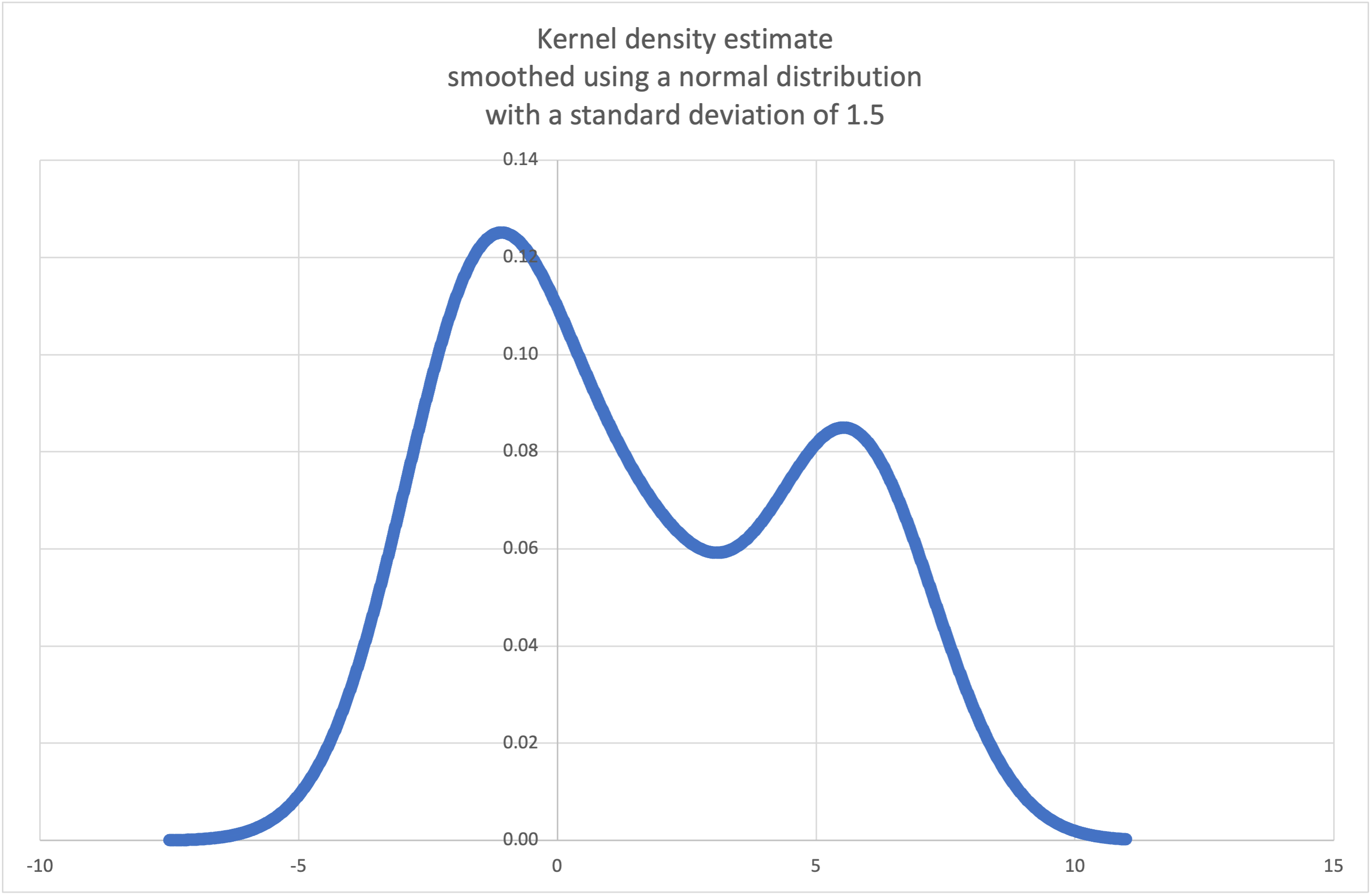
Dodane w wersji 3.13.
- statistics.kde_random(data, h, kernel='normal', *, seed=None)
Return a function that makes a random selection from the estimated probability density function produced by
kde(data, h, kernel).Providing a seed allows reproducible selections. In the future, the values may change slightly as more accurate kernel inverse CDF estimates are implemented. The seed may be an integer, float, str, or bytes.
A
StatisticsErrorwill be raised if the data sequence is empty.Continuing the example for
kde(), we can usekde_random()to generate new random selections from an estimated probability density function:>>> data = [-2.1, -1.3, -0.4, 1.9, 5.1, 6.2] >>> rand = kde_random(data, h=1.5, seed=8675309) >>> new_selections = [rand() for i in range(10)] >>> [round(x, 1) for x in new_selections] [0.7, 6.2, 1.2, 6.9, 7.0, 1.8, 2.5, -0.5, -1.8, 5.6]
Dodane w wersji 3.13.
- statistics.median(data)
Return the median (middle value) of numeric data, using the common „mean of middle two” method. If data is empty,
StatisticsErroris raised. data can be a sequence or iterable.The median is a robust measure of central location and is less affected by the presence of outliers. When the number of data points is odd, the middle data point is returned:
>>> median([1, 3, 5])
3
When the number of data points is even, the median is interpolated by taking the average of the two middle values:
>>> median([1, 3, 5, 7])
4.0
This is suited for when your data is discrete, and you don’t mind that the median may not be an actual data point.
If the data is ordinal (supports order operations) but not numeric (doesn’t support addition), consider using
median_low()ormedian_high()instead.
- statistics.median_low(data)
Return the low median of numeric data. If data is empty,
StatisticsErroris raised. data can be a sequence or iterable.The low median is always a member of the data set. When the number of data points is odd, the middle value is returned. When it is even, the smaller of the two middle values is returned.
>>> median_low([1, 3, 5])
3
>>> median_low([1, 3, 5, 7])
3
Use the low median when your data are discrete and you prefer the median to be an actual data point rather than interpolated.
- statistics.median_high(data)
Return the high median of data. If data is empty,
StatisticsErroris raised. data can be a sequence or iterable.The high median is always a member of the data set. When the number of data points is odd, the middle value is returned. When it is even, the larger of the two middle values is returned.
>>> median_high([1, 3, 5])
3
>>> median_high([1, 3, 5, 7])
5
Use the high median when your data are discrete and you prefer the median to be an actual data point rather than interpolated.
- statistics.median_grouped(data, interval=1.0)
Estimates the median for numeric data that has been grouped or binned around the midpoints of consecutive, fixed-width intervals.
The data can be any iterable of numeric data with each value being exactly the midpoint of a bin. At least one value must be present.
The interval is the width of each bin.
For example, demographic information may have been summarized into consecutive ten-year age groups with each group being represented by the 5-year midpoints of the intervals:
>>> from collections import Counter
>>> demographics = Counter({
...    25: 172,   # 20 to 30 years old
...    35: 484,   # 30 to 40 years old
...    45: 387,   # 40 to 50 years old
...    55:  22,   # 50 to 60 years old
...    65:   6,   # 60 to 70 years old
... })
...
The 50th percentile (median) is the 536th person out of the 1071 member cohort. That person is in the 30 to 40 year old age group.
The regular
median()function would assume that everyone in the tricenarian age group was exactly 35 years old. A more tenable assumption is that the 484 members of that age group are evenly distributed between 30 and 40. For that, we usemedian_grouped():>>> data = list(demographics.elements()) >>> median(data) 35 >>> round(median_grouped(data, interval=10), 1) 37.5
The caller is responsible for making sure the data points are separated by exact multiples of interval. This is essential for getting a correct result. The function does not check this precondition.
Inputs may be any numeric type that can be coerced to a float during the interpolation step.
- statistics.mode(data)
Return the single most common data point from discrete or nominal data. The mode (when it exists) is the most typical value and serves as a measure of central location.
If there are multiple modes with the same frequency, returns the first one encountered in the data. If the smallest or largest of those is desired instead, use
min(multimode(data))ormax(multimode(data)). If the input data is empty,StatisticsErroris raised.modeassumes discrete data and returns a single value. This is the standard treatment of the mode as commonly taught in schools:>>> mode([1, 1, 2, 3, 3, 3, 3, 4]) 3
The mode is unique in that it is the only statistic in this package that also applies to nominal (non-numeric) data:
>>> mode(["red", "blue", "blue", "red", "green", "red", "red"])
'red'
Only hashable inputs are supported. To handle type
set, consider casting tofrozenset. To handle typelist, consider casting totuple. For mixed or nested inputs, consider using this slower quadratic algorithm that only depends on equality tests:max(data, key=data.count).Zmienione w wersji 3.8: Now handles multimodal datasets by returning the first mode encountered. Formerly, it raised
StatisticsErrorwhen more than one mode was found.
- statistics.multimode(data)
Return a list of the most frequently occurring values in the order they were first encountered in the data. Will return more than one result if there are multiple modes or an empty list if the data is empty:
>>> multimode('aabbbbccddddeeffffgg')
['b', 'd', 'f']
>>> multimode('')
[]
Dodane w wersji 3.8.
- statistics.pstdev(data, mu=None)
Return the population standard deviation (the square root of the population variance). See
pvariance()for arguments and other details.>>> pstdev([1.5, 2.5, 2.5, 2.75, 3.25, 4.75]) 0.986893273527251
- statistics.pvariance(data, mu=None)
Return the population variance of data, a non-empty sequence or iterable of real-valued numbers. Variance, or second moment about the mean, is a measure of the variability (spread or dispersion) of data. A large variance indicates that the data is spread out; a small variance indicates it is clustered closely around the mean.
If the optional second argument mu is given, it should be the population mean of the data. It can also be used to compute the second moment around a point that is not the mean. If it is missing or
None(the default), the arithmetic mean is automatically calculated.Use this function to calculate the variance from the entire population. To estimate the variance from a sample, the
variance()function is usually a better choice.Raises
StatisticsErrorif data is empty.Przykłady:
>>> data = [0.0, 0.25, 0.25, 1.25, 1.5, 1.75, 2.75, 3.25]
>>> pvariance(data)
1.25
If you have already calculated the mean of your data, you can pass it as the optional second argument mu to avoid recalculation:
>>> mu = mean(data)
>>> pvariance(data, mu)
1.25
Decimals and Fractions are supported:
>>> from decimal import Decimal as D
>>> pvariance([D("27.5"), D("30.25"), D("30.25"), D("34.5"), D("41.75")])
Decimal('24.815')

>>> from fractions import Fraction as F
>>> pvariance([F(1, 4), F(5, 4), F(1, 2)])
Fraction(13, 72)
Informacja
When called with the entire population, this gives the population variance σ². When called on a sample instead, this is the biased sample variance s², also known as variance with N degrees of freedom.
If you somehow know the true population mean μ, you may use this function to calculate the variance of a sample, giving the known population mean as the second argument. Provided the data points are a random sample of the population, the result will be an unbiased estimate of the population variance.
- statistics.stdev(data, xbar=None)
Return the sample standard deviation (the square root of the sample variance). See
variance()for arguments and other details.>>> stdev([1.5, 2.5, 2.5, 2.75, 3.25, 4.75]) 1.0810874155219827
- statistics.variance(data, xbar=None)
Return the sample variance of data, an iterable of at least two real-valued numbers. Variance, or second moment about the mean, is a measure of the variability (spread or dispersion) of data. A large variance indicates that the data is spread out; a small variance indicates it is clustered closely around the mean.
If the optional second argument xbar is given, it should be the sample mean of data. If it is missing or
None(the default), the mean is automatically calculated.Use this function when your data is a sample from a population. To calculate the variance from the entire population, see
pvariance().Raises
StatisticsErrorif data has fewer than two values.Przykłady:
>>> data = [2.75, 1.75, 1.25, 0.25, 0.5, 1.25, 3.5]
>>> variance(data)
1.3720238095238095
If you have already calculated the sample mean of your data, you can pass it as the optional second argument xbar to avoid recalculation:
>>> m = mean(data)
>>> variance(data, m)
1.3720238095238095
This function does not attempt to verify that you have passed the actual mean as xbar. Using arbitrary values for xbar can lead to invalid or impossible results.
Decimal and Fraction values are supported:
>>> from decimal import Decimal as D
>>> variance([D("27.5"), D("30.25"), D("30.25"), D("34.5"), D("41.75")])
Decimal('31.01875')

>>> from fractions import Fraction as F
>>> variance([F(1, 6), F(1, 2), F(5, 3)])
Fraction(67, 108)
Informacja
This is the sample variance s² with Bessel’s correction, also known as variance with N-1 degrees of freedom. Provided that the data points are representative (e.g. independent and identically distributed), the result should be an unbiased estimate of the true population variance.
If you somehow know the actual population mean μ you should pass it to the
pvariance()function as the mu parameter to get the variance of a sample.
- statistics.quantiles(data, *, n=4, method='exclusive')
Divide data into n continuous intervals with equal probability. Returns a list of
n - 1cut points separating the intervals.Set n to 4 for quartiles (the default). Set n to 10 for deciles. Set n to 100 for percentiles which gives the 99 cuts points that separate data into 100 equal sized groups. Raises
StatisticsErrorif n is not least 1.The data can be any iterable containing sample data. For meaningful results, the number of data points in data should be larger than n. Raises
StatisticsErrorif there is not at least one data point.The cut points are linearly interpolated from the two nearest data points. For example, if a cut point falls one-third of the distance between two sample values,
100and112, the cut-point will evaluate to104.The method for computing quantiles can be varied depending on whether the data includes or excludes the lowest and highest possible values from the population.
The default method is „exclusive” and is used for data sampled from a population that can have more extreme values than found in the samples. The portion of the population falling below the i-th of m sorted data points is computed as
i / (m + 1). Given nine sample values, the method sorts them and assigns the following percentiles: 10%, 20%, 30%, 40%, 50%, 60%, 70%, 80%, 90%.Setting the method to „inclusive” is used for describing population data or for samples that are known to include the most extreme values from the population. The minimum value in data is treated as the 0th percentile and the maximum value is treated as the 100th percentile. The portion of the population falling below the i-th of m sorted data points is computed as
(i - 1) / (m - 1). Given 11 sample values, the method sorts them and assigns the following percentiles: 0%, 10%, 20%, 30%, 40%, 50%, 60%, 70%, 80%, 90%, 100%.# Decile cut points for empirically sampled data >>> data = [105, 129, 87, 86, 111, 111, 89, 81, 108, 92, 110, ... 100, 75, 105, 103, 109, 76, 119, 99, 91, 103, 129, ... 106, 101, 84, 111, 74, 87, 86, 103, 103, 106, 86, ... 111, 75, 87, 102, 121, 111, 88, 89, 101, 106, 95, ... 103, 107, 101, 81, 109, 104] >>> [round(q, 1) for q in quantiles(data, n=10)] [81.0, 86.2, 89.0, 99.4, 102.5, 103.6, 106.0, 109.8, 111.0]
Dodane w wersji 3.8.
Zmienione w wersji 3.13: No longer raises an exception for an input with only a single data point. This allows quantile estimates to be built up one sample point at a time becoming gradually more refined with each new data point.
- statistics.covariance(x, y, /)
Return the sample covariance of two inputs x and y. Covariance is a measure of the joint variability of two inputs.
Both inputs must be of the same length (no less than two), otherwise
StatisticsErroris raised.Przykłady:
>>> x = [1, 2, 3, 4, 5, 6, 7, 8, 9]
>>> y = [1, 2, 3, 1, 2, 3, 1, 2, 3]
>>> covariance(x, y)
0.75
>>> z = [9, 8, 7, 6, 5, 4, 3, 2, 1]
>>> covariance(x, z)
-7.5
>>> covariance(z, x)
-7.5
Dodane w wersji 3.10.
- statistics.correlation(x, y, /, *, method='linear')
Return the Pearson’s correlation coefficient for two inputs. Pearson’s correlation coefficient r takes values between -1 and +1. It measures the strength and direction of a linear relationship.
If method is „ranked”, computes Spearman’s rank correlation coefficient for two inputs. The data is replaced by ranks. Ties are averaged so that equal values receive the same rank. The resulting coefficient measures the strength of a monotonic relationship.
Spearman’s correlation coefficient is appropriate for ordinal data or for continuous data that doesn’t meet the linear proportion requirement for Pearson’s correlation coefficient.
Both inputs must be of the same length (no less than two), and need not to be constant, otherwise
StatisticsErroris raised.Example with Kepler’s laws of planetary motion:
>>> # Mercury, Venus, Earth, Mars, Jupiter, Saturn, Uranus, and  Neptune
>>> orbital_period = [88, 225, 365, 687, 4331, 10_756, 30_687, 60_190]    # days
>>> dist_from_sun = [58, 108, 150, 228, 778, 1_400, 2_900, 4_500] # million km

>>> # Show that a perfect monotonic relationship exists
>>> correlation(orbital_period, dist_from_sun, method='ranked')
1.0

>>> # Observe that a linear relationship is imperfect
>>> round(correlation(orbital_period, dist_from_sun), 4)
0.9882

>>> # Demonstrate Kepler's third law: There is a linear correlation
>>> # between the square of the orbital period and the cube of the
>>> # distance from the sun.
>>> period_squared = [p * p for p in orbital_period]
>>> dist_cubed = [d * d * d for d in dist_from_sun]
>>> round(correlation(period_squared, dist_cubed), 4)
1.0
Dodane w wersji 3.10.
Zmienione w wersji 3.12: Added support for Spearman’s rank correlation coefficient.
- statistics.linear_regression(x, y, /, *, proportional=False)
Return the slope and intercept of simple linear regression parameters estimated using ordinary least squares. Simple linear regression describes the relationship between an independent variable x and a dependent variable y in terms of this linear function:
y = slope * x + intercept + noise
where
slopeandinterceptare the regression parameters that are estimated, andnoiserepresents the variability of the data that was not explained by the linear regression (it is equal to the difference between predicted and actual values of the dependent variable).Both inputs must be of the same length (no less than two), and the independent variable x cannot be constant; otherwise a
StatisticsErroris raised.For example, we can use the release dates of the Monty Python films to predict the cumulative number of Monty Python films that would have been produced by 2019 assuming that they had kept the pace.
>>> year = [1971, 1975, 1979, 1982, 1983]
>>> films_total = [1, 2, 3, 4, 5]
>>> slope, intercept = linear_regression(year, films_total)
>>> round(slope * 2019 + intercept)
16
If proportional is true, the independent variable x and the dependent variable y are assumed to be directly proportional. The data is fit to a line passing through the origin. Since the intercept will always be 0.0, the underlying linear function simplifies to:
y = slope * x + noise
Continuing the example from
correlation(), we look to see how well a model based on major planets can predict the orbital distances for dwarf planets:>>> model = linear_regression(period_squared, dist_cubed, proportional=True) >>> slope = model.slope >>> # Dwarf planets: Pluto, Eris, Makemake, Haumea, Ceres >>> orbital_periods = [90_560, 204_199, 111_845, 103_410, 1_680] # days >>> predicted_dist = [math.cbrt(slope * (p * p)) for p in orbital_periods] >>> list(map(round, predicted_dist)) [5912, 10166, 6806, 6459, 414] >>> [5_906, 10_152, 6_796, 6_450, 414] # actual distance in million km [5906, 10152, 6796, 6450, 414]
Dodane w wersji 3.10.
Zmienione w wersji 3.11: Added support for proportional.
Wyjątki
A single exception is defined:
- exception statistics.StatisticsError
Subclass of
ValueErrorfor statistics-related exceptions.
NormalDist objects
NormalDist is a tool for creating and manipulating normal
distributions of a random variable. It is a
class that treats the mean and standard deviation of data
measurements as a single entity.
Normal distributions arise from the Central Limit Theorem and have a wide range of applications in statistics.
- class statistics.NormalDist(mu=0.0, sigma=1.0)
Returns a new NormalDist object where mu represents the arithmetic mean and sigma represents the standard deviation.
If sigma is negative, raises
StatisticsError.- mean
A read-only property for the arithmetic mean of a normal distribution.
- stdev
A read-only property for the standard deviation of a normal distribution.
- variance
A read-only property for the variance of a normal distribution. Equal to the square of the standard deviation.
- classmethod from_samples(data)
Makes a normal distribution instance with mu and sigma parameters estimated from the data using
fmean()andstdev().The data can be any iterable and should consist of values that can be converted to type
float. If data does not contain at least two elements, raisesStatisticsErrorbecause it takes at least one point to estimate a central value and at least two points to estimate dispersion.
- samples(n, *, seed=None)
Generates n random samples for a given mean and standard deviation. Returns a
listoffloatvalues.If seed is given, creates a new instance of the underlying random number generator. This is useful for creating reproducible results, even in a multi-threading context.
Zmienione w wersji 3.13.
Switched to a faster algorithm. To reproduce samples from previous versions, use
random.seed()andrandom.gauss().
- pdf(x)
Using a probability density function (pdf), compute the relative likelihood that a random variable X will be near the given value x. Mathematically, it is the limit of the ratio
P(x <=
X < x+dx) / dx
as dx approaches zero.The relative likelihood is computed as the probability of a sample occurring in a narrow range divided by the width of the range (hence the word „density”). Since the likelihood is relative to other points, its value can be greater than
1.0.
- cdf(x)
Using a cumulative distribution function (cdf), compute the probability that a random variable X will be less than or equal to x. Mathematically, it is written
P(X <= x).
- inv_cdf(p)
Compute the inverse cumulative distribution function, also known as the quantile function or the percent-point function. Mathematically, it is written
x : P(X <= x) = p.Finds the value x of the random variable X such that the probability of the variable being less than or equal to that value equals the given probability p.
- overlap(other)
Measures the agreement between two normal probability distributions. Returns a value between 0.0 and 1.0 giving the overlapping area for the two probability density functions.
- quantiles(n=4)
Divide the normal distribution into n continuous intervals with equal probability. Returns a list of (n - 1) cut points separating the intervals.
Set n to 4 for quartiles (the default). Set n to 10 for deciles. Set n to 100 for percentiles which gives the 99 cuts points that separate the normal distribution into 100 equal sized groups.
- zscore(x)
Compute the Standard Score describing x in terms of the number of standard deviations above or below the mean of the normal distribution:
(x - mean) / stdev.Dodane w wersji 3.9.
Instances of
NormalDistsupport addition, subtraction, multiplication and division by a constant. These operations are used for translation and scaling. For example:>>> temperature_february = NormalDist(5, 2.5) # Celsius >>> temperature_february * (9/5) + 32 # Fahrenheit NormalDist(mu=41.0, sigma=4.5)
Dividing a constant by an instance of
NormalDistis not supported because the result wouldn’t be normally distributed.Since normal distributions arise from additive effects of independent variables, it is possible to add and subtract two independent normally distributed random variables represented as instances of
NormalDist. For example:>>> birth_weights = NormalDist.from_samples([2.5, 3.1, 2.1, 2.4, 2.7, 3.5]) >>> drug_effects = NormalDist(0.4, 0.15) >>> combined = birth_weights + drug_effects >>> round(combined.mean, 1) 3.1 >>> round(combined.stdev, 1) 0.5
Dodane w wersji 3.8.
Examples and Recipes
Classic probability problems
NormalDist readily solves classic probability problems.
For example, given historical data for SAT exams showing that scores are normally distributed with a mean of 1060 and a standard deviation of 195, determine the percentage of students with test scores between 1100 and 1200, after rounding to the nearest whole number:
>>> sat = NormalDist(1060, 195)
>>> fraction = sat.cdf(1200 + 0.5) - sat.cdf(1100 - 0.5)
>>> round(fraction * 100.0, 1)
18.4
Find the quartiles and deciles for the SAT scores:
>>> list(map(round, sat.quantiles()))
[928, 1060, 1192]
>>> list(map(round, sat.quantiles(n=10)))
[810, 896, 958, 1011, 1060, 1109, 1162, 1224, 1310]
Monte Carlo inputs for simulations
To estimate the distribution for a model that isn’t easy to solve
analytically, NormalDist can generate input samples for a Monte
Carlo simulation:
>>> def model(x, y, z):
...     return (3*x + 7*x*y - 5*y) / (11 * z)
...
>>> n = 100_000
>>> X = NormalDist(10, 2.5).samples(n, seed=3652260728)
>>> Y = NormalDist(15, 1.75).samples(n, seed=4582495471)
>>> Z = NormalDist(50, 1.25).samples(n, seed=6582483453)
>>> quantiles(map(model, X, Y, Z))
[1.4591308524824727, 1.8035946855390597, 2.175091447274739]
Approximating binomial distributions
Normal distributions can be used to approximate Binomial distributions when the sample size is large and when the probability of a successful trial is near 50%.
For example, an open source conference has 750 attendees and two rooms with a 500 person capacity. There is a talk about Python and another about Ruby. In previous conferences, 65% of the attendees preferred to listen to Python talks. Assuming the population preferences haven’t changed, what is the probability that the Python room will stay within its capacity limits?
>>> n = 750             # Sample size
>>> p = 0.65            # Preference for Python
>>> q = 1.0 - p         # Preference for Ruby
>>> k = 500             # Room capacity

>>> # Approximation using the cumulative normal distribution
>>> from math import sqrt
>>> round(NormalDist(mu=n*p, sigma=sqrt(n*p*q)).cdf(k + 0.5), 4)
0.8402

>>> # Exact solution using the cumulative binomial distribution
>>> from math import comb, fsum
>>> round(fsum(comb(n, r) * p**r * q**(n-r) for r in range(k+1)), 4)
0.8402

>>> # Approximation using a simulation
>>> from random import seed, binomialvariate
>>> seed(8675309)
>>> mean(binomialvariate(n, p) <= k for i in range(10_000))
0.8406
Naive bayesian classifier
Normal distributions commonly arise in machine learning problems.
Wikipedia has a nice example of a Naive Bayesian Classifier. The challenge is to predict a person’s gender from measurements of normally distributed features including height, weight, and foot size.
We’re given a training dataset with measurements for eight people. The
measurements are assumed to be normally distributed, so we summarize the data
with NormalDist:
>>> height_male = NormalDist.from_samples([6, 5.92, 5.58, 5.92])
>>> height_female = NormalDist.from_samples([5, 5.5, 5.42, 5.75])
>>> weight_male = NormalDist.from_samples([180, 190, 170, 165])
>>> weight_female = NormalDist.from_samples([100, 150, 130, 150])
>>> foot_size_male = NormalDist.from_samples([12, 11, 12, 10])
>>> foot_size_female = NormalDist.from_samples([6, 8, 7, 9])
Next, we encounter a new person whose feature measurements are known but whose gender is unknown:
>>> ht = 6.0        # height
>>> wt = 130        # weight
>>> fs = 8          # foot size
Starting with a 50% prior probability of being male or female, we compute the posterior as the prior times the product of likelihoods for the feature measurements given the gender:
>>> prior_male = 0.5
>>> prior_female = 0.5
>>> posterior_male = (prior_male * height_male.pdf(ht) *
...                   weight_male.pdf(wt) * foot_size_male.pdf(fs))

>>> posterior_female = (prior_female * height_female.pdf(ht) *
...                     weight_female.pdf(wt) * foot_size_female.pdf(fs))
The final prediction goes to the largest posterior. This is known as the maximum a posteriori or MAP:
>>> 'male' if posterior_male > posterior_female else 'female'
'female'