
statistics --- 數學統計函式
在 3.4 版被加入.
這個模組提供計算數值 (Real-valued) 資料的數學統計函式。
這個模組並非旨在與 NumPy、SciPy 等第三方函式庫,或者像 Minitab、SAS 和 Matlab 等專門設計給專業統計學家的高階統計軟體互相競爭。此模組的目標在於繪圖和科學計算。
除非特別註明,這些函數支援 int、float、Decimal 以及 Fraction。目前不支援其他型別(無論是否為數值型別)。含有混合型別的資料的集合亦是尚未定義,且取決於該型別的實作。若你的輸入資料含有混合型別,你可以考慮使用 map() 來確保結果是一致的,例如:map(float, input_data)。
有些資料集使用 NaN (非數)來表示缺漏的資料。由於 NaN 具有特殊的比較語義,在排序資料或是統計出現次數的統計函數中,會引發意料之外或是未定義的行為。受影響的函數包含 median()、median_low()、 median_high()、 median_grouped()、 mode()、 multimode() 以及 quantiles()。在呼叫這些函數之前,應該先移除 NaN 值:
>>> from statistics import median
>>> from math import isnan
>>> from itertools import filterfalse

>>> data = [20.7, float('NaN'),19.2, 18.3, float('NaN'), 14.4]
>>> sorted(data)  # This has surprising behavior
[20.7, nan, 14.4, 18.3, 19.2, nan]
>>> median(data)  # This result is unexpected
16.35

>>> sum(map(isnan, data))    # Number of missing values
2
>>> clean = list(filterfalse(isnan, data))  # Strip NaN values
>>> clean
[20.7, 19.2, 18.3, 14.4]
>>> sorted(clean)  # Sorting now works as expected
[14.4, 18.3, 19.2, 20.7]
>>> median(clean)       # This result is now well defined
18.75
平均值與中央位置量數
這些函式計算來自一個母體或樣本的平均值或代表值。
資料的算術平均數(平均值)。 |
|
快速浮點數算數平均數,可調整權重。 |
|
資料的幾何平均數。 |
|
資料的調和平均數。 |
|
Estimate the probability density distribution of the data. |
|
Random sampling from the PDF generated by kde(). |
|
資料的中位數(中間值)。 |
|
資料中較小的中位數。 |
|
資料中較大的中位數。 |
|
分組資料的中位數(第 50 百分位數)。 |
|
離散 (discrete) 或名目 (nomial) 資料中的眾數(出現次數最多次的值),只回傳一個。 |
|
離散或名目資料中的眾數(出現次數最多次的值)組成的 list。 |
|
將資料分成數個具有相等機率的區間,即分位數 (quantile)。 |
離度 (spread) 的測量
這些函式計算母體或樣本偏離平均值的程度。
資料的母體標準差。 |
|
資料的母體變異數。 |
|
資料的樣本標準差。 |
|
資料的樣本變異數。 |
兩個輸入之間的關係統計
這些函式計算兩個輸入之間的關係統計數據。
兩變數的樣本共變異數。 |
|
Pearson 與 Spearman 相關係數 (correlation coefficient)。 |
|
簡單線性迴歸的斜率和截距。 |
函式細節
註:這些函數並不要求輸入的資料必須排序過。為了閱讀方便,大部份的範例仍已排序過。
- statistics.mean(data)
回傳 data 的樣本算數平均數,輸入可為一個 sequence 或者 iterable。
算數平均數為資料總和除以資料點的數目。他通常被稱為「平均值」,儘管它只是眾多不同的數學平均值之一。它是衡量資料集中位置的一種指標。
若 data 為空,則會引發
StatisticsError。使用範例:
>>> mean([1, 2, 3, 4, 4])
2.8
>>> mean([-1.0, 2.5, 3.25, 5.75])
2.625

>>> from fractions import Fraction as F
>>> mean([F(3, 7), F(1, 21), F(5, 3), F(1, 3)])
Fraction(13, 21)

>>> from decimal import Decimal as D
>>> mean([D("0.5"), D("0.75"), D("0.625"), D("0.375")])
Decimal('0.5625')
備註
平均值強烈受到離群值 (outliers) 的影響,且不一定能當作這些資料點的典型範例。若要使用更穩健但效率較低的集中趨勢 (central tendency) 度量,請參考
median()。樣本平均數提供了對真實母體平均數的不偏估計 (unbiased estimate),所以從所有可能的樣本中取平均值時,
mean(sample)會收斂至整個母體的真實平均值。若 data 為整個母體而非單一樣本,則mean(data)等同於計算真實的母體平均數 μ。
- statistics.fmean(data, weights=None)
將 data 轉換為浮點數並計算其算數平均數。
這個函式運算比
mean()更快,並且它總是回傳一個float。data 可以是一個 sequence 或者 iterable。如果輸入的資料為空,則引發StatisticsError。>>> fmean([3.5, 4.0, 5.25]) 4.25
支援選擇性的加權。例如,一位教授以 20% 的比重計算小考分數,20% 的比重計算作業分數,30% 的比重計算期中考試分數,以及 30% 的比重計算期末考試分數:
>>> grades = [85, 92, 83, 91]
>>> weights = [0.20, 0.20, 0.30, 0.30]
>>> fmean(grades, weights)
87.6
如果有提供 weights,它必須與 data 長度相同,否則將引發
ValueError。在 3.8 版被加入.
在 3.11 版的變更: 新增 weights 的支援。
- statistics.geometric_mean(data)
將 data 轉換成浮點數並計算其幾何平均數。
幾何平均數使用數值的乘積(與之對照,算數平均數使用的是數值的和)來表示 data 的集中趨勢或典型值。
若輸入的資料集為空、包含零、包含負值,則引發
StatisticsError。data 可為 sequence 或者 iterable。目前沒有特別為了精確結果而特別多下什麼工夫。(然而,未來或許會有。)
>>> round(geometric_mean([54, 24, 36]), 1)
36.0
在 3.8 版被加入.
- statistics.harmonic_mean(data, weights=None)
回傳 data 的調和平均數。data 可為實數 (real-valued) sequence 或者 iterable。如果省略 weights 或者 weights 為
None,則假設各權重相等。調和平均數是資料的倒數 (reciprocal) 經過
mean()運算過後的倒數。例如,三個數 a,b 與 c 的調和平均數等於3/(1/a + 1/b + 1/c)。若其中一個值為零,結果將為零。調和平均數是一種平均數,是衡量資料中心位置的一種方法。它通常用於計算比率 (ratio) 或率 (rate) 的平均,例如速率(speed)。
假設一輛汽車以時速 40 公里的速率行駛 10 公里,然後再以時速 60 公里的速率行駛 10 公里,求汽車的平均速率?
>>> harmonic_mean([40, 60])
48.0
假設一輛汽車以時速 40 公里的速率行駛 5 公里,然後在交通順暢時,加速到時速 60 公里,以此速度行駛剩下的 30 公里。求汽車的平均速率?
>>> harmonic_mean([40, 60], weights=[5, 30])
56.0
若 data 為空、含有任何小於零的元素、或者加權總和不為正數,則引發
StatisticsError。目前的演算法設計為,若在輸入當中遇到零,則會提前退出。這意味著後續的輸入並未進行有效性檢查。(這種行為在未來可能會改變。)
在 3.6 版被加入.
在 3.10 版的變更: 新增 weights 的支援。
- statistics.kde(data, h, kernel='normal', *, cumulative=False)
Kernel Density Estimation (KDE): Create a continuous probability density function or cumulative distribution function from discrete samples.
The basic idea is to smooth the data using a kernel function. to help draw inferences about a population from a sample.
The degree of smoothing is controlled by the scaling parameter h which is called the bandwidth. Smaller values emphasize local features while larger values give smoother results.
The kernel determines the relative weights of the sample data points. Generally, the choice of kernel shape does not matter as much as the more influential bandwidth smoothing parameter.
Kernels that give some weight to every sample point include normal (gauss), logistic, and sigmoid.
Kernels that only give weight to sample points within the bandwidth include rectangular (uniform), triangular, parabolic (epanechnikov), quartic (biweight), triweight, and cosine.
If cumulative is true, will return a cumulative distribution function.
若 data 為空,則引發
StatisticsError。維基百科有一個範例,我們可以使用
kde()來從一個小樣本生成並繪製估計的機率密度函數:>>> sample = [-2.1, -1.3, -0.4, 1.9, 5.1, 6.2] >>> f_hat = kde(sample, h=1.5) >>> xarr = [i/100 for i in range(-750, 1100)] >>> yarr = [f_hat(x) for x in xarr]
xarr和yarr中的點可用於繪製 PDF 圖: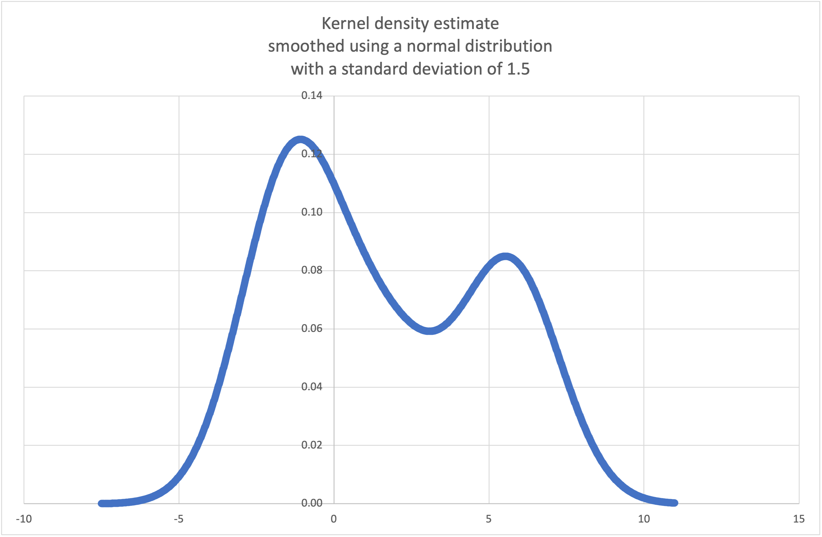
在 3.13 版被加入.
- statistics.kde_random(data, h, kernel='normal', *, seed=None)
Return a function that makes a random selection from the estimated probability density function produced by
kde(data, h, kernel).Providing a seed allows reproducible selections. In the future, the values may change slightly as more accurate kernel inverse CDF estimates are implemented. The seed may be an integer, float, str, or bytes.
若 data 為空,則引發
StatisticsError。Continuing the example for
kde(), we can usekde_random()to generate new random selections from an estimated probability density function:>>> data = [-2.1, -1.3, -0.4, 1.9, 5.1, 6.2] >>> rand = kde_random(data, h=1.5, seed=8675309) >>> new_selections = [rand() for i in range(10)] >>> [round(x, 1) for x in new_selections] [0.7, 6.2, 1.2, 6.9, 7.0, 1.8, 2.5, -0.5, -1.8, 5.6]
在 3.13 版被加入.
- statistics.median(data)
使用常見的「中間兩數取平均」方法回傳數值資料的中位數 (中間值)。若 data 為空,則會引發
StatisticsError。data 可為一個 sequence 或者 iterable。中位數是一種穩健的衡量資料中心位置的方法,較不易被離群值影響。當資料點數量為奇數時,會回傳中間的資料點:
>>> median([1, 3, 5])
3
當資料點數量為偶數時,中位數透過中間兩個值的平均數來插值計算:
>>> median([1, 3, 5, 7])
4.0
若你的資料為離散資料,並且你不介意中位數可能並非真實的資料點,那這函式適合你。
若你的資料為順序 (ordinal) 資料(支援排序操作)但並非數值型(不支援加法),可以考慮改用
median_low()或是median_high()代替。
- statistics.median_low(data)
回傳數值型資料的低中位數 (low median)。若 data 為空,則引發
StatisticsError。data 可為 sequence 或者 iterable。低中位數一定會在原本的資料集當中。當資料點數量為奇數時,回傳中間值。當數量為偶數時,回傳兩個中間值當中較小的值。
>>> median_low([1, 3, 5])
3
>>> median_low([1, 3, 5, 7])
3
當你的資料為離散資料,且你希望中位數是實際的資料點而不是插值時,可以用低中位數。
- statistics.median_high(data)
回傳數值型資料的高中位數 (high median)。若 data 為空,則引發
StatisticsError。data 可為 sequence 或者 iterable。高中位數一定會在原本的資料集當中。當資料點數量為奇數時,回傳中間值。當數量為偶數時,回傳兩個中間值當中較大的值。
>>> median_high([1, 3, 5])
3
>>> median_high([1, 3, 5, 7])
5
當你的資料為離散資料,且你希望中位數是實際的資料點而不是插值時,可以用高中位數。
- statistics.median_grouped(data, interval=1.0)
Estimates the median for numeric data that has been grouped or binned around the midpoints of consecutive, fixed-width intervals.
The data can be any iterable of numeric data with each value being exactly the midpoint of a bin. At least one value must be present.
The interval is the width of each bin.
For example, demographic information may have been summarized into consecutive ten-year age groups with each group being represented by the 5-year midpoints of the intervals:
>>> from collections import Counter
>>> demographics = Counter({
...    25: 172,   # 20 to 30 years old
...    35: 484,   # 30 to 40 years old
...    45: 387,   # 40 to 50 years old
...    55:  22,   # 50 to 60 years old
...    65:   6,   # 60 to 70 years old
... })
...
The 50th percentile (median) is the 536th person out of the 1071 member cohort. That person is in the 30 to 40 year old age group.
The regular
median()function would assume that everyone in the tricenarian age group was exactly 35 years old. A more tenable assumption is that the 484 members of that age group are evenly distributed between 30 and 40. For that, we usemedian_grouped():>>> data = list(demographics.elements()) >>> median(data) 35 >>> round(median_grouped(data, interval=10), 1) 37.5
The caller is responsible for making sure the data points are separated by exact multiples of interval. This is essential for getting a correct result. The function does not check this precondition.
Inputs may be any numeric type that can be coerced to a float during the interpolation step.
- statistics.mode(data)
回傳離散或名目 data 中出現次數最多次的值,只回傳一個。眾數(如果存在)是最典型的值,並用來衡量資料的中心位置。
若有多個出現次數相同的眾數,則回傳在 data 中最先出現的眾數。如果希望回傳其中最小或最大的眾數,可以使用
min(multimode(data))或max(multimode(data))。如果輸入的 data 為空,則會引發StatisticsError。mode假定為離散資料,並回傳單一的值。這也是一般學校教授的標準眾數定義:>>> mode([1, 1, 2, 3, 3, 3, 3, 4]) 3
眾數特別之處在於它是此套件中唯一也適用於名目(非數值型)資料的統計量:
>>> mode(["red", "blue", "blue", "red", "green", "red", "red"])
'red'
Only hashable inputs are supported. To handle type
set, consider casting tofrozenset. To handle typelist, consider casting totuple. For mixed or nested inputs, consider using this slower quadratic algorithm that only depends on equality tests:max(data, key=data.count).在 3.8 版的變更: 現在,遇到資料中有多個眾數時,會回傳第一個遇到的眾數。在以前,當找到大於一個眾數時,會引發
StatisticsError。
- statistics.multimode(data)
回傳一個 list,其組成為 data 中出現次數最多次的值,並按照它們在 data 中首次出現的順序排列。如果有多個眾數,將會回傳所有結果。若 data 為空,則回傳空的 list:
>>> multimode('aabbbbccddddeeffffgg')
['b', 'd', 'f']
>>> multimode('')
[]
在 3.8 版被加入.
- statistics.pstdev(data, mu=None)
回傳母體標準差(即母體變異數的平方根)。有關引數以及其他細節,請參見
pvariance()。>>> pstdev([1.5, 2.5, 2.5, 2.75, 3.25, 4.75]) 0.986893273527251
- statistics.pvariance(data, mu=None)
回傳 data 的母體變異數。data 可為非空實數 sequence 或者 iterable。變異數,或者以平均數為中心的二階動差,用於衡量資料的變異性(離度或分散程度)。變異數大表示資料分散,變異數小表示資料集中在平均數附近。
若有傳入選擇性的第二個引數 mu,該引數應該要是 data 的母體平均值 (population mean)。它也可以用於計算非以平均值為中心的第二動差。如果沒有傳入此引數或者引數為
None(預設值),則自動計算資料的算數平均數。使用此函式來計算整個母體的變異數。如果要從樣本估算變異數,
variance()通常是較好的選擇。若 data 為空,則引發
StatisticsError。範例:
>>> data = [0.0, 0.25, 0.25, 1.25, 1.5, 1.75, 2.75, 3.25]
>>> pvariance(data)
1.25
如果已經計算出資料的平均值,你可以將其作為選擇性的第二個引數 mu 傳遞以避免重新計算:
>>> mu = mean(data)
>>> pvariance(data, mu)
1.25
支援小數 (decimal) 與分數 (fraction):
>>> from decimal import Decimal as D
>>> pvariance([D("27.5"), D("30.25"), D("30.25"), D("34.5"), D("41.75")])
Decimal('24.815')

>>> from fractions import Fraction as F
>>> pvariance([F(1, 4), F(5, 4), F(1, 2)])
Fraction(13, 72)
備註
當在整個母體上呼叫此函式時,會回傳母體變異數 σ²。當在樣本上呼叫此函式時,會回傳有偏差的樣本變異數 s²,也就是具有 N 個自由度的變異數。
若你以某種方式知道真正的母體平均數 μ,你可以將一個已知的母體平均數作為第二個引數提供給此函式,用以計算樣本的變異數。只要資料點是母體的隨機樣本,結果將是母體變異數的不偏估計。
- statistics.stdev(data, xbar=None)
回傳樣本標準差(即樣本變異數的平方根)。有關引數以及其他細節,請參見
variance()。>>> stdev([1.5, 2.5, 2.5, 2.75, 3.25, 4.75]) 1.0810874155219827
- statistics.variance(data, xbar=None)
回傳 data 的樣本變異數。data 為兩個值以上的實數 iterable。變異數,或者以平均數為中心的二階動差,用於衡量資料的變異性(離度或分散程度)。變異數大表示資料分散,變異數小表示資料集中在平均數附近。
若有傳入選擇性的第二個引數 xbar,它應該是 data 的樣本平均值 (sample mean)。如果沒有傳入或者為
None(預設值),則自動計算資料的平均值。當你的資料是來自母體的樣本時,請使用此函式。若要從整個母體計算變異數,請參見
pvariance()。若 data 內少於兩個值,則引發
StatisticsError。範例:
>>> data = [2.75, 1.75, 1.25, 0.25, 0.5, 1.25, 3.5]
>>> variance(data)
1.3720238095238095
如果已經計算出資料的樣本平均值,你可以將其作為選擇性的第二個引數 mu 傳遞以避免重新計算:
>>> m = mean(data)
>>> variance(data, m)
1.3720238095238095
此函式不會驗證你傳入的 xbar 是否為實際的平均數。傳入任意的 xbar 會導致無效或不可能的結果。
支援小數 (decimal) 與分數 (fraction):
>>> from decimal import Decimal as D
>>> variance([D("27.5"), D("30.25"), D("30.25"), D("34.5"), D("41.75")])
Decimal('31.01875')

>>> from fractions import Fraction as F
>>> variance([F(1, 6), F(1, 2), F(5, 3)])
Fraction(67, 108)
備註
這是經過 Bessel 校正 (Bessel's correction) 後的樣本變異數 s² ,又稱為自由度為 N-1 的變異數。只要資料點具有代表性(例如:獨立且具有相同分布),結果應該會是對真實母體變異數的不偏估計。
若你剛好知道真正的母體平均數 μ,你應該將其作為 mu 參數傳入
pvariance()函式來計算樣本變異數。
- statistics.quantiles(data, *, n=4, method='exclusive')
將 data 分成 n 個具有相等機率的連續區間。回傳一個包含
n - 1個用於切分各區間的分隔點的 list。將 n 設為 4 以表示四分位數 (quartile) (預設值)。將 n 設置為 100 表示百分位數 (percentile),這將給出 99 個分隔點將 data 分成 100 個大小相等的組。如果 n 不是至少為 1,則引發
StatisticsError。data 可以是包含樣本資料的任何 iterable。為了取得有意義的結果,data 中的資料點數量應大於 n。如果連一個資料點都沒有,則引發
StatisticsError。分隔點是從兩個最近的資料點線性內插值計算出來的。舉例來說,如果分隔點落在兩個樣本值
100與112之間的距離三分之一處,則分隔點的值將為104。計算分位數的 method 可以根據 data 是否包含或排除來自母體的最小與最大可能的值而改變。
預設的 method 是 "exclusive",用於從可能找到比樣本更極端的值的母體中抽樣的樣本資料。對於 m 個已排序的資料點,計算出低於 i-th 的部分為
i / (m + 1)。給定九個樣本資料,此方法將對資料排序且計算下列百分位數:10%、20%、30%、40%、50%、60%、70%、80%、90%。若將 method 設為 "inclusive",則用於描述母體或者已知包含母體中最極端值的樣本資料。在 data 中的最小值被視為第 0 百分位數,最大值為第 100 百分位數。對於 m 個已排序的資料點,計算出低於 i-th 的部分為
(i - 1) / (m - 1)。給定十一個個樣本資料,此方法將對資料排序且計算下列百分位數:0%、10%、20%、30%、40%、50%、60%、70%、80%、90%、100%。# Decile cut points for empirically sampled data >>> data = [105, 129, 87, 86, 111, 111, 89, 81, 108, 92, 110, ... 100, 75, 105, 103, 109, 76, 119, 99, 91, 103, 129, ... 106, 101, 84, 111, 74, 87, 86, 103, 103, 106, 86, ... 111, 75, 87, 102, 121, 111, 88, 89, 101, 106, 95, ... 103, 107, 101, 81, 109, 104] >>> [round(q, 1) for q in quantiles(data, n=10)] [81.0, 86.2, 89.0, 99.4, 102.5, 103.6, 106.0, 109.8, 111.0]
在 3.8 版被加入.
在 3.13 版的變更: No longer raises an exception for an input with only a single data point. This allows quantile estimates to be built up one sample point at a time becoming gradually more refined with each new data point.
- statistics.covariance(x, y, /)
回傳兩輸入 x 與 y 的樣本共變異數 (sample covariance)。共變異數是衡量兩輸入的聯合變異性 (joint variability) 的指標。
兩輸入必須具有相同長度(至少兩個),否則會引發
StatisticsError。範例:
>>> x = [1, 2, 3, 4, 5, 6, 7, 8, 9]
>>> y = [1, 2, 3, 1, 2, 3, 1, 2, 3]
>>> covariance(x, y)
0.75
>>> z = [9, 8, 7, 6, 5, 4, 3, 2, 1]
>>> covariance(x, z)
-7.5
>>> covariance(z, x)
-7.5
在 3.10 版被加入.
- statistics.correlation(x, y, /, *, method='linear')
回傳兩輸入的 Pearson 相關係數 (Pearson’s correlation coefficient)。Pearson 相關係數 r 的值介於 -1 與 +1 之間。它衡量線性關係的強度與方向。
如果 method 為 "ranked",則計算兩輸入的 Spearman 等級相關係數 (Spearman’s rank correlation coefficient)。資料將被取代為等級。平手的情況則取平均,令相同的值排名也相同。所得係數衡量單調關係 (monotonic relationship) 的強度。
Spearman 相關係數適用於順序型資料,或者不符合 Pearson 相關係數要求的線性比例關係的連續型 (continuous) 資料。
兩輸入必須具有相同長度(至少兩個),且不須為常數,否則會引發
StatisticsError。以 Kepler 行星運動定律為例:
>>> # Mercury, Venus, Earth, Mars, Jupiter, Saturn, Uranus, and  Neptune
>>> orbital_period = [88, 225, 365, 687, 4331, 10_756, 30_687, 60_190]    # days
>>> dist_from_sun = [58, 108, 150, 228, 778, 1_400, 2_900, 4_500] # million km

>>> # Show that a perfect monotonic relationship exists
>>> correlation(orbital_period, dist_from_sun, method='ranked')
1.0

>>> # Observe that a linear relationship is imperfect
>>> round(correlation(orbital_period, dist_from_sun), 4)
0.9882

>>> # Demonstrate Kepler's third law: There is a linear correlation
>>> # between the square of the orbital period and the cube of the
>>> # distance from the sun.
>>> period_squared = [p * p for p in orbital_period]
>>> dist_cubed = [d * d * d for d in dist_from_sun]
>>> round(correlation(period_squared, dist_cubed), 4)
1.0
在 3.10 版被加入.
在 3.12 版的變更: 新增了對 Spearman 等級相關係數的支援。
- statistics.linear_regression(x, y, /, *, proportional=False)
回傳使用普通最小平方法 (ordinary least square) 估計出的簡單線性迴歸 (simple linear regression) 參數中的斜率 (slope) 與截距 (intercept)。簡單線性迴歸描述自變數 (independent variable) x 與應變數 (dependent variable) y 之間的關係,用以下的線性函式表示:
y = slope * x + intercept + noise
其中
slope和intercept是被估計的迴歸參數,而noise表示由線性迴歸未解釋的資料變異性(它等於應變數的預測值與實際值之差)。兩輸入必須具有相同長度(至少兩個),且自變數 x 不得為常數,否則會引發
StatisticsError。舉例來說,我們可以使用 Monty Python 系列電影的上映日期來預測至 2019 年為止,假設他們保持固定的製作速度,應該會產生的 Monty Python 電影的累計數量。
>>> year = [1971, 1975, 1979, 1982, 1983]
>>> films_total = [1, 2, 3, 4, 5]
>>> slope, intercept = linear_regression(year, films_total)
>>> round(slope * 2019 + intercept)
16
若將 proportional 設為 True,則假設自變數 x 與應變數 y 是直接成比例的,資料座落在通過原點的一直線上。由於 intercept 始終為 0.0,因此線性函式可簡化如下:
y = slope * x + noise
繼續
correlation()中的範例,我們看看基於主要行星的模型可以如何很好地預測矮行星的軌道距離:>>> model = linear_regression(period_squared, dist_cubed, proportional=True) >>> slope = model.slope >>> # 矮行星: 冥王星、 鬩神星、 鳥神星、 妊神星、 穀神星 >>> orbital_periods = [90_560, 204_199, 111_845, 103_410, 1_680] # 天數 >>> predicted_dist = [math.cbrt(slope * (p * p)) for p in orbital_periods] >>> list(map(round, predicted_dist)) [5912, 10166, 6806, 6459, 414] >>> [5_906, 10_152, 6_796, 6_450, 414] # 以百萬公里為單位的實際距離 [5906, 10152, 6796, 6450, 414]
在 3.10 版被加入.
在 3.11 版的變更: 新增 proportional 的支援。
例外
定義了一個單一的例外:
- exception statistics.StatisticsError
ValueError的子類別,用於和統計相關的例外。
NormalDist 物件
NormalDist 是一種用於建立與操作隨機變數 (random variable) 的常態分布的工具。它是一個將量測資料的平均數與標準差視為單一實體的類別。
常態分布源自於中央極限定理 (Central Limit Theorem),在統計學中有著廣泛的應用。
- class statistics.NormalDist(mu=0.0, sigma=1.0)
此方法會回傳一個新 NormalDist 物件,其中 mu 代表算數平均數而 sigma 代表標準差。
若 sigma 為負值,則引發
StatisticsError。- classmethod from_samples(data)
利用
fmean()與stdev()函式,估計 data 的 mu 與 sigma 參數,建立一個常態分布的實例。data 可以是任何 iterable,並應包含可以轉換為
float的值。若 data 沒有包含至少兩個以上的元素在內,則引發StatisticsError,因為至少需要一個點來估計中央值且至少需要兩個點來估計分散情形。
- samples(n, *, seed=None)
給定平均值與標準差,產生 n 個隨機樣本。回傳一個由
float組成的list。若有給定 seed,則會建立一個以此為基礎的亂數產生器實例。這對於建立可重現的結果很有幫助,即使在多執行緒情境下也是如此。
在 3.13 版的變更.
Switched to a faster algorithm. To reproduce samples from previous versions, use
random.seed()andrandom.gauss().
- pdf(x)
利用機率密度函數 (probability density function, pdf) 計算隨機變數 X 接近給定值 x 的相對概度 (relative likelihood)。數學上,它是比率
P(x <= X < x+dx) / dx在 dx 趨近於零時的極限值。相對概度是樣本出現在狹窄範圍的機率,除以該範圍的寬度(故稱為「密度」)計算而得。由於概度是相對於其它點,故其值可大於
1.0。
- cdf(x)
利用累積分布函式 (cumulative distribution function, cdf) 計算隨機變數 X 小於或等於 x 的機率。數學上,它記為
P(X <= x)。
- inv_cdf(p)
計算反累計分布函式 (inverse cumulative distribution function),也稱為分位數函式 (quantile function) 或者百分率點 (percent-point) 函式。數學上記為
x : P(X <= x) = p。找出一個值 x,使得隨機變數 X 小於或等於該值的機率等於給定的機率 p。
- overlap(other)
衡量兩常態分布之間的一致性。回傳一個介於 0.0 與 1.0 之間的值,表示兩機率密度函式的重疊區域。
- quantiles(n=4)
將常態分布分割成 n 個具有相等機率的連續區間。回傳一個 list,包含 (n-1) 個切割區間的分隔點。
將 n 設定為 4 表示四分位數(預設值)。將 n 設定為 10 表示十分位數。將 n 設定為 100 表示百分位數,這會產生 99 個分隔點,將常態分布切割成大小相等的群組。
- zscore(x)
計算標準分數 (Standard Score),用以描述在常態分布中,x 高出或低於平均數幾個標準差:
(x - mean) / stdev。在 3.9 版被加入.
NormalDist的實例支援對常數的加法、減法、乘法與除法。這些操作用於平移與縮放。例如:>>> temperature_february = NormalDist(5, 2.5) # 攝氏 >>> temperature_february * (9/5) + 32 # 華氏 NormalDist(mu=41.0, sigma=4.5)
不支援將常數除以
NormalDist的實例,因為結果將不符合常態分布。由於常態分布源自於自變數的加法效應 (additive effects),因此可以將兩個獨立的常態分布隨機變數相加與相減,並且表示為
NormalDist的實例。例如:>>> birth_weights = NormalDist.from_samples([2.5, 3.1, 2.1, 2.4, 2.7, 3.5]) >>> drug_effects = NormalDist(0.4, 0.15) >>> combined = birth_weights + drug_effects >>> round(combined.mean, 1) 3.1 >>> round(combined.stdev, 1) 0.5
在 3.8 版被加入.
範例與錦囊妙計
經典機率問題
NormalDist 可以輕易地解決經典的機率問題。
例如,給定 SAT 測驗的歷史資料,顯示成績為平均 1060、標準差 195 的常態分布。我們要求出分數在 1100 與 1200 之間(四捨五入至最接近的整數)的學生的百分比:
>>> sat = NormalDist(1060, 195)
>>> fraction = sat.cdf(1200 + 0.5) - sat.cdf(1100 - 0.5)
>>> round(fraction * 100.0, 1)
18.4
>>> list(map(round, sat.quantiles()))
[928, 1060, 1192]
>>> list(map(round, sat.quantiles(n=10)))
[810, 896, 958, 1011, 1060, 1109, 1162, 1224, 1310]
用於模擬的蒙地卡羅 (Monte Carlo) 輸入
欲估計一個不易透過解析方法求解的模型的分布,NormalDist 可以產生輸入樣本以進行蒙地卡羅模擬:
>>> def model(x, y, z):
...     return (3*x + 7*x*y - 5*y) / (11 * z)
...
>>> n = 100_000
>>> X = NormalDist(10, 2.5).samples(n, seed=3652260728)
>>> Y = NormalDist(15, 1.75).samples(n, seed=4582495471)
>>> Z = NormalDist(50, 1.25).samples(n, seed=6582483453)
>>> quantiles(map(model, X, Y, Z))
[1.4591308524824727, 1.8035946855390597, 2.175091447274739]
近似二項分布
當樣本數量夠大,且試驗成功的機率接近 50%,可以使用常態分布來近似二項分布 (Binomial distributions)。
例如,一場有 750 位參加者的開源研討會中,有兩間可容納 500 人的會議室。一場是關於 Python 的講座,另一場則是關於 Ruby 的。在過去的會議中,有 65% 的參加者傾向參與 Python 講座。假設參與者的偏好沒有改變,那麼 Python 會議室未超過自身容量限制的機率是?
>>> n = 750             # Sample size
>>> p = 0.65            # Preference for Python
>>> q = 1.0 - p         # Preference for Ruby
>>> k = 500             # Room capacity

>>> # Approximation using the cumulative normal distribution
>>> from math import sqrt
>>> round(NormalDist(mu=n*p, sigma=sqrt(n*p*q)).cdf(k + 0.5), 4)
0.8402

>>> # Exact solution using the cumulative binomial distribution
>>> from math import comb, fsum
>>> round(fsum(comb(n, r) * p**r * q**(n-r) for r in range(k+1)), 4)
0.8402

>>> # Approximation using a simulation
>>> from random import seed, binomialvariate
>>> seed(8675309)
>>> mean(binomialvariate(n, p) <= k for i in range(10_000))
0.8406
單純貝氏分類器 (Naive bayesian classifier)
常態分布常在機器學習問題中出現。
維基百科有個 Naive Bayesian Classifier 的優良範例。課題為從身高、體重與鞋子尺寸等符合常態分布的特徵量測值中判斷一個人的性別。
給定一組包含八個人的量測值的訓練資料集。假設這些量測值服從常態分布,我們可以利用 NormalDist 來總結資料:
>>> height_male = NormalDist.from_samples([6, 5.92, 5.58, 5.92])
>>> height_female = NormalDist.from_samples([5, 5.5, 5.42, 5.75])
>>> weight_male = NormalDist.from_samples([180, 190, 170, 165])
>>> weight_female = NormalDist.from_samples([100, 150, 130, 150])
>>> foot_size_male = NormalDist.from_samples([12, 11, 12, 10])
>>> foot_size_female = NormalDist.from_samples([6, 8, 7, 9])
接著,我們遇到一個新的人,他的特徵量測值已知,但性別未知:
>>> ht = 6.0        # height
>>> wt = 130        # weight
>>> fs = 8          # foot size
從可能為男性或女性的 50% 先驗機率 (prior probability) 為開端,我們將後驗機率 (posterior probability) 計算為先驗機率乘以給定性別下,各特徵量測值的概度乘積:
>>> prior_male = 0.5
>>> prior_female = 0.5
>>> posterior_male = (prior_male * height_male.pdf(ht) *
...                   weight_male.pdf(wt) * foot_size_male.pdf(fs))

>>> posterior_female = (prior_female * height_female.pdf(ht) *
...                     weight_female.pdf(wt) * foot_size_female.pdf(fs))
最終的預測結果將取決於最大的後驗機率。這被稱為最大後驗機率 (maximum a posteriori) 或者 MAP:
>>> 'male' if posterior_male > posterior_female else 'female'
'female'