statistics — 수학 통계 함수

Added in version 3.4.

소스 코드: Lib/statistics.py

---

이 모듈은 숫자 (Real 값) 데이터의 수학적 통계를 계산하는 함수를 제공합니다.

이 모듈은 NumPy, SciPy와 같은 제삼자 라이브러리나 Minitab, SAS 및 Matlab과 같은 통계 전문가를 대상으로 하는 완전한 기능의 통계 패키지와 경쟁하기 위한 것이 아닙니다. 그래프를 그릴 수 있는 과학 계산기의 수준을 목표로 합니다.

달리 명시되지 않는 한, 이 함수는 int, float, decimal.Decimal 및 fractions.Fraction을 지원합니다. 다른 형(숫자 계층에 있든 없든)에서의 동작은 현재 지원되지 않습니다. 여러 형의 컬렉션도 정의되지 않으며 구현에 따라 다릅니다. 입력 데이터가 혼합형으로 구성되었으면, map()을 사용하여 일관된 결과를 보장 할 수 있습니다, 예를 들어 map(float, input_data).

Some datasets use NaN (not a number) values to represent missing data. Since NaNs have unusual comparison semantics, they cause surprising or undefined behaviors in the statistics functions that sort data or that count occurrences. The functions affected are median(), median_low(), median_high(), median_grouped(), mode(), multimode(), and quantiles(). The NaN values should be stripped before calling these functions:

>>> from statistics import median
>>> from math import isnan
>>> from itertools import filterfalse

>>> data = [20.7, float('NaN'),19.2, 18.3, float('NaN'), 14.4]
>>> sorted(data)  # 놀라운 행동을 보입니다
[20.7, nan, 14.4, 18.3, 19.2, nan]
>>> median(data)  # 예상치 못한 결과입니다
16.35

>>> sum(map(isnan, data))    # 누락된 값의 수
2
>>> clean = list(filterfalse(isnan, data))  # NaN 값을 제거합니다
>>> clean
[20.7, 19.2, 18.3, 14.4]
>>> sorted(clean)  # 정렬이 이제 예상대로 작동합니다
[14.4, 18.3, 19.2, 20.7]
>>> median(clean)       # 이제 결과가 잘 정의됩니다
18.75

평균과 중심 위치의 측정

이 함수는 모집단(population)이나 표본(sample)에서 평균이나 최빈값을 계산합니다.

mean()	데이터의 산술 평균(arithmetic mean) ( “average”).
fmean()	빠른, 부동 소수점 산술 평균, 선택적 가중치 적용.
geometric_mean()	데이터의 기하 평균(geometric mean).
harmonic_mean()	데이터의 조화 평균(harmonic mean).
kde()	Estimate the probability density distribution of the data.
kde_random()	Random sampling from the PDF generated by kde().
median()	데이터의 중앙값(median) (중간값).
median_low()	데이터의 낮은 중앙값(low median).
median_high()	데이터의 높은 중앙값(high median).
median_grouped()	그룹화된 데이터의 중앙값 (50번째 백분위 수)
mode()	이산(discrete) 또는 범주(nominal) 데이터의 단일 최빈값(mode) (가장 흔한 값)
multimode()	이산 또는 범주 데이터의 최빈값(mode) (가장 흔한 값) 리스트.
quantiles()	데이터를 같은 확률을 갖는 구간으로 나눕니다.

분산 측정

이 함수는 모집단이나 표본이 평균값에서 벗어나는 정도를 측정합니다.

pstdev()	데이터의 모집단 표준 편차(population standard deviation).
pvariance()	데이터의 모집단 분산(population variance).
stdev()	데이터의 표본 표준 편차(sample standard deviation).
variance()	데이터의 표본 분산(sample variance).

Statistics for relations between two inputs

These functions calculate statistics regarding relations between two inputs.

covariance()	두 변수의 표본 공분산.
correlation()	Pearson and Spearman’s correlation coefficients.
linear_regression()	Slope and intercept for simple linear regression.

함수 세부 사항

참고: 함수에 전달되는 데이터가 정렬될 필요는 없습니다. 하지만, 읽기 쉽도록 대부분 예제는 정렬된 시퀀스를 보여줍니다.

statistics.mean(data)

시퀀스나 이터러블일 수 있는 data의 표본 산술 평균을 반환합니다.

산술 평균은 데이터의 합을 데이터 포인트 수로 나눈 값입니다. 흔히 “평균”이라고 합니다만, 많은 수학적 평균 중 하나일 뿐입니다. 데이터의 중심 위치에 대한 측정(measure)입니다.

data가 비어 있으면, StatisticsError가 발생합니다.

사용 예:

>>> mean([1, 2, 3, 4, 4])
2.8
>>> mean([-1.0, 2.5, 3.25, 5.75])
2.625

>>> from fractions import Fraction as F
>>> mean([F(3, 7), F(1, 21), F(5, 3), F(1, 3)])
Fraction(13, 21)

>>> from decimal import Decimal as D
>>> mean([D("0.5"), D("0.75"), D("0.625"), D("0.375")])
Decimal('0.5625')

참고

평균은 특이치의 영향을 많이 받으며, 반드시 데이터 포인트의 전형적인 예는 아닙니다. 비록 효율성은 떨어지지만, 더 강인한, 중심 경향성의 측정은, median()을 참조하십시오.

표본 평균은 실제 모집단 평균의 편향되지 않은(unbiased) 추정치를 제공합니다. 즉, 가능한 모든 표본에 대해 평균을 취하면, mean(sample)은 전체 모집단의 실제 평균에 수렴합니다. data가 표본이 아닌 전체 모집단을 나타낸다면, mean(data)는 실제 모집단 평균 μ를 계산하는 것과 동등합니다.

statistics.fmean(data, weights=None)

data를 float로 변환하고 산술 평균을 계산합니다.

mean() 함수보다 빠르게 실행되며 항상 float를 반환합니다. data는 시퀀스나 이터러블일 수 있습니다. 입력 data가 비어 있으면 StatisticsError를 발생시킵니다.

>>> fmean([3.5, 4.0, 5.25])
4.25

Optional weighting is supported. For example, a professor assigns a grade for a course by weighting quizzes at 20%, homework at 20%, a midterm exam at 30%, and a final exam at 30%:

>>> grades = [85, 92, 83, 91]
>>> weights = [0.20, 0.20, 0.30, 0.30]
>>> fmean(grades, weights)
87.6

If weights is supplied, it must be the same length as the data or a ValueError will be raised.

Added in version 3.8.

버전 3.11에서 변경: Added support for weights.

statistics.geometric_mean(data)

data를 float로 변환하고 기하 평균(geometric mean)을 계산합니다.

기하 평균은 값의 곱을 사용하는 data의 중심 경향(central tendency)이나 대표값(typical value)을 나타냅니다 (합을 사용하는 산술 평균과 달리).

입력 data가 비어 있거나, 0을 포함하거나, 음수 값을 포함하면 StatisticsError를 발생시킵니다. data는 시퀀스나 이터러블일 수 있습니다.

정확한 결과를 얻기 위해 특별한 노력을 기울이지는 않습니다. (하지만, 향후 변경될 수 있습니다.)

>>> round(geometric_mean([54, 24, 36]), 1)
36.0

Added in version 3.8.

statistics.harmonic_mean(data, weights=None)

실숫값 숫자의 시퀀스나 이터러블인 data의 조화 평균(harmonic mean)을 반환합니다. weights가 생략되거나 None이면, 균등 가중치를 가정합니다.

조화 평균은 데이터의 역수의 산술 mean()의 역수입니다. 예를 들어, 세 a, b 및 c 값의 조화 평균은 3/(1/a + 1/b + 1/c)와 동등합니다. 값 중 하나가 0이면, 결과는 0입니다.

조화 평균은 데이터의 중심 위치의 측정인 평균의 한가지 유형입니다. 예를 들어 속도와 같은 비율(ratio)이나 율(rate)을 평균할 때 종종 적합합니다.

자동차가 40km/hr로 10km를 주행한 다음, 60km/hr로 10km를 주행한다고 가정해 봅시다. 평균 속도는 얼마입니까?

>>> harmonic_mean([40, 60])
48.0

Suppose a car travels 40 km/hr for 5 km, and when traffic clears, speeds-up to 60 km/hr for the remaining 30 km of the journey. What is the average speed?

>>> harmonic_mean([40, 60], weights=[5, 30])
56.0

data가 비어 있거나, 0보다 작은 값이 있거나, 가중 합이 양수가 아니면 StatisticsError가 발생합니다.

현재 알고리즘은 입력에서 0을 만나면 조기 종료됩니다. 이는 후속 입력의 유효성을 검사하지 않았음을 의미합니다. (이 동작은 나중에 변경될 수 있습니다.)

Added in version 3.6.

버전 3.10에서 변경: Added support for weights.

statistics.kde(data, h, kernel='normal', *, cumulative=False)

Kernel Density Estimation (KDE): Create a continuous probability density function or cumulative distribution function from discrete samples.

The basic idea is to smooth the data using a kernel function. to help draw inferences about a population from a sample.

The degree of smoothing is controlled by the scaling parameter h which is called the bandwidth. Smaller values emphasize local features while larger values give smoother results.

The kernel determines the relative weights of the sample data points. Generally, the choice of kernel shape does not matter as much as the more influential bandwidth smoothing parameter.

Kernels that give some weight to every sample point include normal (gauss), logistic, and sigmoid.

Kernels that only give weight to sample points within the bandwidth include rectangular (uniform), triangular, parabolic (epanechnikov), quartic (biweight), triweight, and cosine.

If cumulative is true, will return a cumulative distribution function.

data 시퀀스가 비어 있으면 StatisticsError를 발생시킵니다.

Wikipedia has an example where we can use kde() to generate and plot a probability density function estimated from a small sample:

>>> sample = [-2.1, -1.3, -0.4, 1.9, 5.1, 6.2]
>>> f_hat = kde(sample, h=1.5)
>>> xarr = [i/100 for i in range(-750, 1100)]
>>> yarr = [f_hat(x) for x in xarr]

The points in xarr and yarr can be used to make a PDF plot: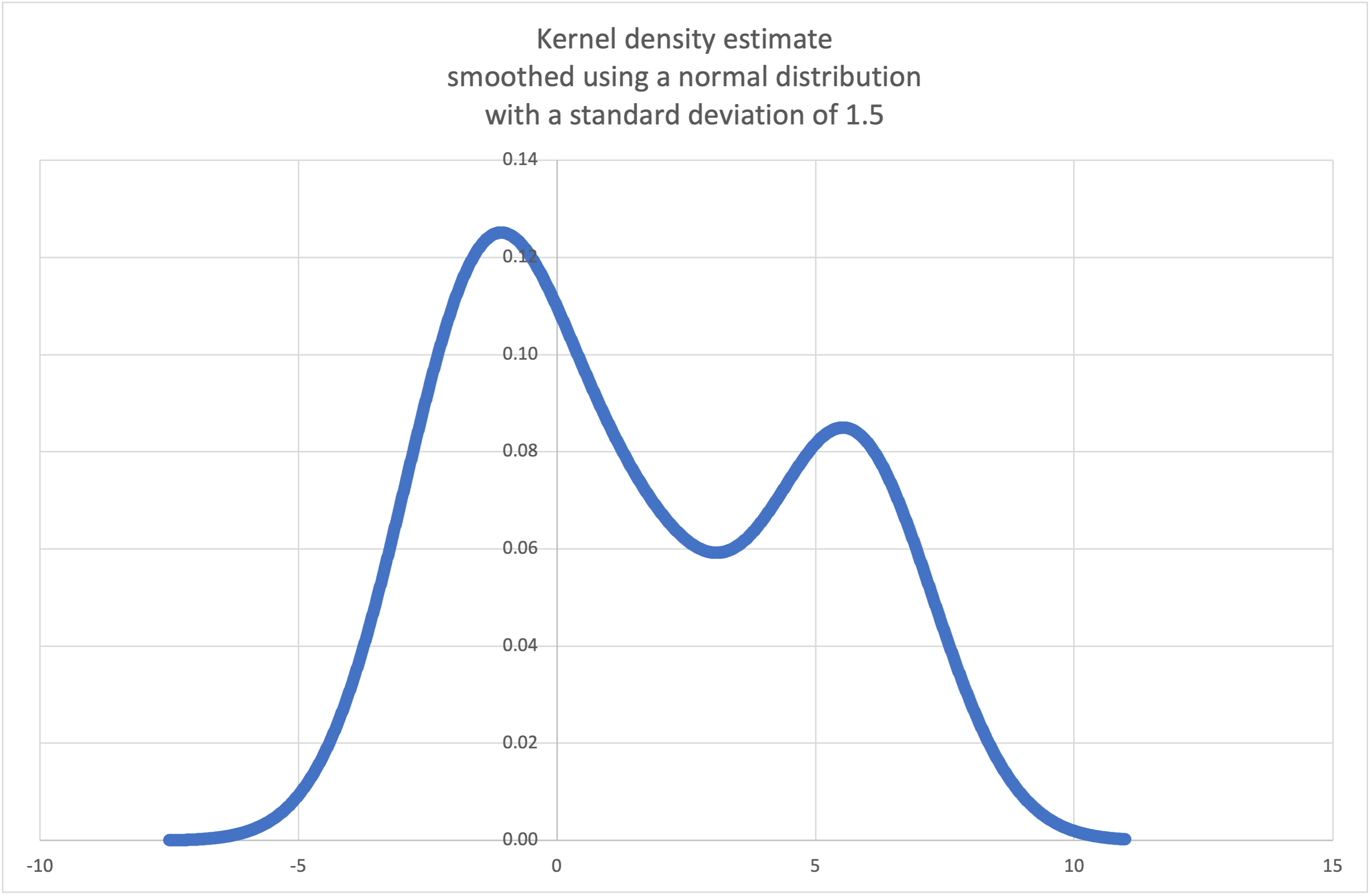

Added in version 3.13.

statistics.kde_random(data, h, kernel='normal', *, seed=None)

Return a function that makes a random selection from the estimated probability density function produced by kde(data, h, kernel).

Providing a seed allows reproducible selections. In the future, the values may change slightly as more accurate kernel inverse CDF estimates are implemented. The seed may be an integer, float, str, or bytes.

data 시퀀스가 비어 있으면 StatisticsError를 발생시킵니다.

Continuing the example for kde(), we can use kde_random() to generate new random selections from an estimated probability density function:

>>> data = [-2.1, -1.3, -0.4, 1.9, 5.1, 6.2]
>>> rand = kde_random(data, h=1.5, seed=8675309)
>>> new_selections = [rand() for i in range(10)]
>>> [round(x, 1) for x in new_selections]
[0.7, 6.2, 1.2, 6.9, 7.0, 1.8, 2.5, -0.5, -1.8, 5.6]

Added in version 3.13.

statistics.median(data)

일반적인 “중간 2개의 평균” 방법을 사용하여, 숫자 data의 중앙값(중간값)을 반환합니다. data가 비어 있으면, StatisticsError가 발생합니다. data는 시퀀스나 이터러블일 수 있습니다.

중앙값은 중심 위치에 대한 강인한 측정이며, 특이치가 있을 때 영향을 덜 받습니다. 데이터 포인트 수가 홀수면, 가운데 데이터 포인트가 반환됩니다:

>>> median([1, 3, 5])
3

데이터 포인트 수가 짝수면, 중앙값은 두 가운데 값의 평균을 취하여 보간됩니다:

>>> median([1, 3, 5, 7])
4.0

데이터가 이산(discrete)적이고, 중앙값이 실제 데이터 포인트가 아니라도 상관없을 때 적합합니다.

데이터가 순서는 있지만 (대소 비교 지원) 숫자가 아니면 (덧셈을 지원하지 않음), 대신 median_low()나 median_high()를 사용하는 것을 고려하십시오.

statistics.median_low(data)

숫자 데이터의 낮은 중앙값을 반환합니다. data가 비어 있으면 StatisticsError가 발생합니다. data는 시퀀스나 이터러블일 수 있습니다.

낮은 중앙값은 항상 데이터 세트의 멤버입니다. 데이터 포인트 수가 홀수이면 중간값이 반환됩니다. 짝수이면, 두 중간값 중 작은 값이 반환됩니다.

>>> median_low([1, 3, 5])
3
>>> median_low([1, 3, 5, 7])
3

데이터가 이산(discrete)적이고 보간된 값이 아닌 실제 데이터 포인트를 중앙값으로 선호할 때 낮은 중앙값을 사용하십시오.

statistics.median_high(data)

데이터의 높은 중앙값을 반환합니다. data가 비어 있으면 StatisticsError가 발생합니다. data는 시퀀스나 이터러블일 수 있습니다.

높은 중앙값은 항상 데이터 세트의 멤버입니다. 데이터 포인트 수가 홀수이면 중간값이 반환됩니다. 짝수이면, 두 중간값 중 큰 값이 반환됩니다.

>>> median_high([1, 3, 5])
3
>>> median_high([1, 3, 5, 7])
5

데이터가 이산(discrete)적이고 보간된 값이 아닌 실제 데이터 포인트를 중앙값으로 선호할 때 높은 중앙값을 사용하십시오.

statistics.median_grouped(data, interval=1.0)

Estimates the median for numeric data that has been grouped or binned around the midpoints of consecutive, fixed-width intervals.

The data can be any iterable of numeric data with each value being exactly the midpoint of a bin. At least one value must be present.

The interval is the width of each bin.

For example, demographic information may have been summarized into consecutive ten-year age groups with each group being represented by the 5-year midpoints of the intervals:

>>> from collections import Counter
>>> demographics = Counter({
...    25: 172,   # 20 에서 30 세
...    35: 484,   # 30 에서 40 세
...    45: 387,   # 40 에서 50 세
...    55:  22,   # 50 에서 60 세
...    65:   6,   # 60 에서 70 세
... })
...

The 50th percentile (median) is the 536th person out of the 1071 member cohort. That person is in the 30 to 40 year old age group.

The regular median() function would assume that everyone in the tricenarian age group was exactly 35 years old. A more tenable assumption is that the 484 members of that age group are evenly distributed between 30 and 40. For that, we use median_grouped():

>>> data = list(demographics.elements())
>>> median(data)
35
>>> round(median_grouped(data, interval=10), 1)
37.5

The caller is responsible for making sure the data points are separated by exact multiples of interval. This is essential for getting a correct result. The function does not check this precondition.

Inputs may be any numeric type that can be coerced to a float during the interpolation step.

statistics.mode(data)

이산(discrete)적이거나 범주(nominal)적인 data에서 가장 흔한 단일 데이터 포인트를 반환합니다. 최빈값(mode)은 (존재할 때) 가장 흔한 값이며 중심 위치의 측정으로 기능합니다.

같은 빈도의 여러 최빈값이 있으면, data에서 처음 발견된 첫 번째 값을 반환합니다. 여러 최빈값 중 가장 작거나 가장 큰 값이 필요하면 대신 min(multimode(data))나 max(multimode(data))를 사용하십시오. 입력 data가 비어 있으면, StatisticsError가 발생합니다.

mode는 이산 데이터를 가정하고 단일 값을 반환합니다. 이것이 학교에서 일반적으로 가르치는 최빈값의 표준적인 처리입니다:

>>> mode([1, 1, 2, 3, 3, 3, 3, 4])
3

최빈값은 범주(nominal)적 (숫자가 아닌) 데이터에도 적용되는 이 패키지에 있는 유일한 통계라는 점에서 특별합니다:

>>> mode(["red", "blue", "blue", "red", "green", "red", "red"])
'red'

Only hashable inputs are supported. To handle type set, consider casting to frozenset. To handle type list, consider casting to tuple. For mixed or nested inputs, consider using this slower quadratic algorithm that only depends on equality tests: max(data, key=data.count).

버전 3.8에서 변경: 이제 첫 번째 최빈값을 모드를 반환하여 다봉(multimodal) 데이터 세트를 처리합니다. 이전에는, 둘 이상의 최빈값이 발견되면 StatisticsError가 발생했습니다.

statistics.multimode(data)

data에서 먼저 발견되는 순서대로 가장 자주 등장하는 값의 리스트를 반환합니다. 여러 최빈값이 있으면 둘 이상의 결과를 반환하고, data가 비어 있으면 빈 리스트를 반환합니다:

>>> multimode('aabbbbccddddeeffffgg')
['b', 'd', 'f']
>>> multimode('')
[]

Added in version 3.8.

statistics.pstdev(data, mu=None)

모집단 표준 편차(모집단 분산의 제곱근)를 반환합니다. 인자와 기타 세부 사항은 pvariance()를 참조하십시오.

>>> pstdev([1.5, 2.5, 2.5, 2.75, 3.25, 4.75])
0.986893273527251

statistics.pvariance(data, mu=None)

실수 숫자의 비어있지 않은 시퀀스나 이터러블인 data의 모집단 분산을 반환합니다. 분산(또는 평균에 대한 이차 모멘트)은 데이터 변동성(퍼진 정도)의 측정입니다. 큰 분산은 데이터가 퍼져 있음을 나타냅니다; 작은 분산은 평균 주변에 군집되어 있음을 나타냅니다.

선택적 두 번째 인자 mu가 제공되면, data의 모집단 평균이어야 합니다. 평균이 아닌 점을 기준으로 이차 모멘트를 계산하는 데에도 사용할 수 있습니다. 누락되었거나 None(기본값)이면, 산술 평균이 자동으로 계산됩니다.

이 함수를 사용하여 전체 모집단의 분산을 계산하십시오. 표본으로 분산을 추정하려면, 일반적으로 variance() 함수가 더 좋은 선택입니다.

data가 비어 있으면 StatisticsError를 발생시킵니다.

예:

>>> data = [0.0, 0.25, 0.25, 1.25, 1.5, 1.75, 2.75, 3.25]
>>> pvariance(data)
1.25

데이터의 평균을 이미 계산했다면, 재계산을 피하고자 선택적인 두 번째 인자 mu로 전달할 수 있습니다:

>>> mu = mean(data)
>>> pvariance(data, mu)
1.25

Decimal과 Fraction이 지원됩니다:

>>> from decimal import Decimal as D
>>> pvariance([D("27.5"), D("30.25"), D("30.25"), D("34.5"), D("41.75")])
Decimal('24.815')

>>> from fractions import Fraction as F
>>> pvariance([F(1, 4), F(5, 4), F(1, 2)])
Fraction(13, 72)

참고

전체 모집단으로 호출하면, 모집단 분산 σ²을 줍니다. 대신 표본으로 호출하면, 편향된(biased) 표본 분산 s²이 됩니다, N 자유도의 분산이라고도 합니다.

실제 모집단 평균 μ를 어떻게든 알고 있다면, 알려진 모집단 평균을 두 번째 인자로 지정해서, 이 함수를 사용하여 표본의 분산을 계산할 수 있습니다. 데이터 포인트가 모집단의 무작위 표본이면, 결과는 모집단 분산의 편향 없는(unbiased) 추정치가 됩니다.

statistics.stdev(data, xbar=None)

표본 표준 편차(표본 분산의 제곱근)를 반환합니다. 인자와 기타 세부 사항은 variance()를 참조하십시오.

>>> stdev([1.5, 2.5, 2.5, 2.75, 3.25, 4.75])
1.0810874155219827

statistics.variance(data, xbar=None)

적어도 두 개의 실수 숫자를 제공하는 이터러블인 data의 표본 분산을 반환합니다. 분산(또는 평균에 대한 이차 모멘트)은 데이터 변동성(퍼진 정도)의 측정입니다. 큰 분산은 데이터가 퍼져 있음을 나타냅니다; 작은 분산은 평균 주변에 군집되어 있음을 나타냅니다.

선택적 두 번째 인자 xbar가 제공되면, data의 표본 평균이어야 합니다. 누락되었거나 None(기본값)이면, 평균은 자동으로 계산됩니다.

데이터가 모집단의 표본이면 이 함수를 사용하십시오. 전체 모집단의 분산을 계산하려면, pvariance()를 참조하십시오.

data의 두 개 미만의 값을 갖고 있으면 StatisticsError를 발생시킵니다.

예:

>>> data = [2.75, 1.75, 1.25, 0.25, 0.5, 1.25, 3.5]
>>> variance(data)
1.3720238095238095

데이터의 표본 평균을 이미 계산했다면, 재계산을 피하고자 선택적인 두 번째 인자 xbar로 전달할 수 있습니다:

>>> m = mean(data)
>>> variance(data, m)
1.3720238095238095

이 함수는 실제 평균을 xbar로 전달했는지 확인하지 않습니다. xbar에 임의의 값을 사용하면 결과가 유효하지 않거나 불가능한 값일 수 있습니다.

Decimal과 Fraction 값이 지원됩니다:

>>> from decimal import Decimal as D
>>> variance([D("27.5"), D("30.25"), D("30.25"), D("34.5"), D("41.75")])
Decimal('31.01875')

>>> from fractions import Fraction as F
>>> variance([F(1, 6), F(1, 2), F(5, 3)])
Fraction(67, 108)

참고

이것은 베셀 보정(Bessel’s correction)을 적용한 표본 분산 s² 입니다, N-1 자유도의 분산이라고도 합니다. 데이터 포인트가 대표적(예를 들어, 독립적이고 동일하게 분포된)이라면, 결과는 실제 모집단 분산의 편향 없는(unbiased) 추정치가 되어야 합니다.

실제 모집단 평균 μ를 어떻게든 알고 있다면 mu 매개 변수로 pvariance() 함수에 전달하여 표본의 분산을 구해야 합니다.

statistics.quantiles(data, *, n=4, method='exclusive')

data를 같은 확률을 갖는 n 개의 연속 구간으로 나눕니다. 구간을 분할하는 n - 1개의 절단 점(cut point) 리스트를 반환합니다.

사분위는 n을 4로 설정하십시오 (기본값). 십분위는 n을 10으로 설정하십시오. 백분위는 n을 100으로 설정하십시오. 그러면 data를 100개의 같은 크기 그룹으로 분할하는 99개의 절단 점이 제공됩니다. n이 1 미만이면 StatisticsError를 발생시킵니다.

data는 표본 데이터를 포함하는 모든 이터러블일 수 있습니다. 의미 있는 결과를 얻으려면, data의 데이터 포인트 수가 n보다 커야 합니다. 최소한 하나의 데이터 포인트도 없으면 StatisticsError를 발생시킵니다.

절단 점은 가장 가까운 두 개의 데이터 포인트에서 선형 보간됩니다. 예를 들어, 절단 점이 두 표본 값 100과 112 사이의 거리로 1/3 지점에 해당하면, 절단 점은 104로 평가됩니다.

균등 분위(quantile) 계산 방법(method)은 data가 모집단에서 가능한 최젓값과 최곳값을 포함하는지 제외하는지에 따라 달라질 수 있습니다.

기본 method는 “exclusive”이며, 표본에서 발견되는 것보다 더 극단적인 값을 가질 수 있는 모집단에서 표본 추출된 데이터에 사용됩니다. m 개의 정렬된 데이터 포인트의 i-번째 아래로 떨어지는 모집단 부분은 i / (m + 1)로 계산됩니다. 9개의 표본 값을 주면, 이 방법은 그들을 정렬한 다음, 다음과 같은 백분위를 할당합니다: 10%, 20%, 30%, 40%, 50%, 60%, 70%, 80%, 90%.

method를 “inclusive”로 설정하는 것은 모집단 데이터를 기술하거나 모집단의 가장 극단적인 값을 포함하는 것으로 알려진 표본에 사용됩니다. data의 최솟값은 0번째 백분위 수로 취급되고 최댓값은 100번째 백분위 수로 취급됩니다. m 개의 정렬된 데이터 포인트의 i-번째 아래로 떨어지는 모집단 부분은 (i - 1) / (m - 1)로 계산됩니다. 11개의 표본 값을 주면, 이 방법은 그들을 정렬한 다음, 다음과 같은 백분위를 할당합니다: 0%, 10%, 20%, 30%, 40%, 50%, 60%, 70%, 80%, 90%, 100%.

# 경험적으로 표본 추출된 데이터에 대한 십 분위 절단 점
>>> data = [105, 129, 87, 86, 111, 111, 89, 81, 108, 92, 110,
...         100, 75, 105, 103, 109, 76, 119, 99, 91, 103, 129,
...         106, 101, 84, 111, 74, 87, 86, 103, 103, 106, 86,
...         111, 75, 87, 102, 121, 111, 88, 89, 101, 106, 95,
...         103, 107, 101, 81, 109, 104]
>>> [round(q, 1) for q in quantiles(data, n=10)]
[81.0, 86.2, 89.0, 99.4, 102.5, 103.6, 106.0, 109.8, 111.0]

Added in version 3.8.

버전 3.13에서 변경: No longer raises an exception for an input with only a single data point. This allows quantile estimates to be built up one sample point at a time becoming gradually more refined with each new data point.

statistics.covariance(x, y, /)

Return the sample covariance of two inputs x and y. Covariance is a measure of the joint variability of two inputs.

Both inputs must be of the same length (no less than two), otherwise StatisticsError is raised.

예:

>>> x = [1, 2, 3, 4, 5, 6, 7, 8, 9]
>>> y = [1, 2, 3, 1, 2, 3, 1, 2, 3]
>>> covariance(x, y)
0.75
>>> z = [9, 8, 7, 6, 5, 4, 3, 2, 1]
>>> covariance(x, z)
-7.5
>>> covariance(z, x)
-7.5

Added in version 3.10.

statistics.correlation(x, y, /, *, method='linear')

Return the Pearson’s correlation coefficient for two inputs. Pearson’s correlation coefficient r takes values between -1 and +1. It measures the strength and direction of a linear relationship.

If method is “ranked”, computes Spearman’s rank correlation coefficient for two inputs. The data is replaced by ranks. Ties are averaged so that equal values receive the same rank. The resulting coefficient measures the strength of a monotonic relationship.

Spearman’s correlation coefficient is appropriate for ordinal data or for continuous data that doesn’t meet the linear proportion requirement for Pearson’s correlation coefficient.

Both inputs must be of the same length (no less than two), and need not to be constant, otherwise StatisticsError is raised.

Example with Kepler’s laws of planetary motion:

>>> # 수성, 금성, 지구, 화성, 목성, 토성, 천왕성 및  해왕성
>>> orbital_period = [88, 225, 365, 687, 4331, 10_756, 30_687, 60_190]    # days
>>> dist_from_sun = [58, 108, 150, 228, 778, 1_400, 2_900, 4_500] # million km

>>> # 완벽한 단조 관계가 존재함을 보입니다
>>> correlation(orbital_period, dist_from_sun, method='ranked')
1.0

>>> # 선형 관계가 불완전함을 관찰합니다
>>> round(correlation(orbital_period, dist_from_sun), 4)
0.9882

>>> # 케플러의 제3법칙을 시연합니다: 궤도 주기의 제곱과
>>> # 태양으로부터의 거리 세제곱 간에 선형 상관관계가
>>> # 존재합니다.
>>> period_squared = [p * p for p in orbital_period]
>>> dist_cubed = [d * d * d for d in dist_from_sun]
>>> round(correlation(period_squared, dist_cubed), 4)
1.0

Added in version 3.10.

버전 3.12에서 변경: Added support for Spearman’s rank correlation coefficient.

statistics.linear_regression(x, y, /, *, proportional=False)

Return the slope and intercept of simple linear regression parameters estimated using ordinary least squares. Simple linear regression describes the relationship between an independent variable x and a dependent variable y in terms of this linear function:

y = slope * x + intercept + noise

where slope and intercept are the regression parameters that are estimated, and noise represents the variability of the data that was not explained by the linear regression (it is equal to the difference between predicted and actual values of the dependent variable).

Both inputs must be of the same length (no less than two), and the independent variable x cannot be constant; otherwise a StatisticsError is raised.

For example, we can use the release dates of the Monty Python films to predict the cumulative number of Monty Python films that would have been produced by 2019 assuming that they had kept the pace.

>>> year = [1971, 1975, 1979, 1982, 1983]
>>> films_total = [1, 2, 3, 4, 5]
>>> slope, intercept = linear_regression(year, films_total)
>>> round(slope * 2019 + intercept)
16

If proportional is true, the independent variable x and the dependent variable y are assumed to be directly proportional. The data is fit to a line passing through the origin. Since the intercept will always be 0.0, the underlying linear function simplifies to:

y = slope * x + noise

Continuing the example from correlation(), we look to see how well a model based on major planets can predict the orbital distances for dwarf planets:

>>> model = linear_regression(period_squared, dist_cubed, proportional=True)
>>> slope = model.slope

>>> # 왜행성:             명왕성,    에리스,     마케마케,    하우메아,    세레스
>>> orbital_periods = [90_560, 204_199, 111_845, 103_410, 1_680]  # 일
>>> predicted_dist = [math.cbrt(slope * (p * p)) for p in orbital_periods]
>>> list(map(round, predicted_dist))
[5912, 10166, 6806, 6459, 414]

>>> [5_906, 10_152, 6_796, 6_450, 414]  # 백만 km 단위의 실제 거리
[5906, 10152, 6796, 6450, 414]

Added in version 3.10.

버전 3.11에서 변경: Added support for proportional.

예외

하나의 예외가 정의됩니다:

exception statistics.StatisticsError

통계 관련 예외를 위한 ValueError의 서브 클래스.

NormalDist 객체

NormalDist는 무작위 변수의 정규 분포를 만들고 조작하기 위한 도구입니다. 데이터 측정의 평균과 표준 편차를 단일 엔티티로 취급하는 클래스입니다.

정규 분포는 중심 극한 정리(Central Limit Theorem)에서 도출되며 통계에서 광범위하게 응용됩니다.

class statistics.NormalDist(mu=0.0, sigma=1.0)

mu가 산술 평균을 나타내고 sigma가 표준 편차를 나타내는 새 NormalDist 객체를 반환합니다.

sigma가 음수이면 StatisticsError를 발생시킵니다.

mean

정규 분포의 산술 평균에 대한 읽기 전용 프로퍼티.

median

정규 분포의 중앙값에 대한 읽기 전용 프로퍼티.

mode

정규 분포의 최빈값에 대한 읽기 전용 프로퍼티.

stdev

정규 분포의 표준 편차에 대한 읽기 전용 프로퍼티.

variance

정규 분포의 분산에 대한 읽기 전용 프로퍼티. 표준 편차의 제곱과 같습니다.

classmethod from_samples(data)

fmean()과 stdev()를 사용해서 data에서 추정된 mu와 sigma 매개 변수로 정규 분포 인스턴스를 만듭니다.

data는 임의의 이터러블일 수 있으며 float 형으로 변환될 수 있는 값으로 구성되어야 합니다. data가 두 개 이상의 값을 포함하지 않으면 StatisticsError를 발생시키는데, 중심 값을 추정하는 데 적어도 한 점이 필요하고 분산을 추정하는 데 적어도 두 점이 필요하기 때문입니다.

samples(n, *, seed=None)

주어진 평균과 표준 편차로 n 개의 무작위 표본을 생성합니다. float 값의 list를 반환합니다.

seed가 제공되면, 하부 난수 생성기의 새 인스턴스를 만듭니다. 이는 다중 스레딩 문맥에서도, 재현 가능한 결과를 만드는 데 유용합니다.

버전 3.13에서 변경.

Switched to a faster algorithm. To reproduce samples from previous versions, use random.seed() and random.gauss().

pdf(x)

확률 밀도 함수(pdf)를 사용하여, 무작위 변수 X가 주어진 값 x에 가까울 상대적 가능도(likelihood)를 계산합니다. 수학적으로, 비율 P(x <= X < x+dx) / dx의 dx가 0으로 접근할 때의 극한값입니다.

상대적 가능도는 좁은 구간에 표본이 발생할 수 있는 확률을 구간의 너비로 나눈 값으로 계산됩니다 (그래서 “밀도”라고 합니다). 가능도는 다른 점에 상대적이기 때문에, 1.0보다 클 수 있습니다.

cdf(x)

누적 분포 함수 (cdf)를 사용하여, 무작위 변수 X가 x보다 작거나 같을 확률을 계산합니다. 수학적으로, P(X <= x)라고 씁니다.

inv_cdf(p)

분위 함수(quantile function)나 백분위 수(percent-point) 함수라고도 하는 역 누적 분포 함수를 계산합니다. 수학적으로, x : P(X <= x) = p라고 씁니다.

변수가 x보다 작거나 같을 확률이 주어진 확률 p와 같아지도록 하는 무작위 변수 X의 값 x를 찾습니다.

overlap(other)

두 정규 확률 분포 간의 일치를 측정합니다. 두 확률 밀도 함수가 겹치는 영역의 면적을 제공하는 0.0과 1.0 사이의 값을 반환합니다.

quantiles(n=4)

정규 분포를 같은 확률을 갖는 n 개의 연속 구간으로 나눕니다. 구간을 분할하는 (n - 1)개의 절단 점(cut point) 리스트를 반환합니다.

사분위는 n을 4로 설정하십시오 (기본값). 십분위는 n을 10으로 설정하십시오. 백분위는 n을 100으로 설정하십시오, 그러면 정규 분포를 100개의 같은 크기 그룹으로 분할하는 99개의 절단 점이 제공됩니다.

zscore(x)

정규 분포의 평균 위나 아래의 표준 편차 수로 x를 설명하는 표준 점수(Standard Score)를 계산합니다: (x - mean) / stdev.

Added in version 3.9.

NormalDist의 인스턴스는 상수에 의한 덧셈, 뺄셈, 곱셈 및 나눗셈을 지원합니다. 이러한 연산은 이동(translation)과 확대(scaling)에 사용됩니다. 예를 들면:

>>> temperature_february = NormalDist(5, 2.5)             # 섭씨
>>> temperature_february * (9/5) + 32                     # 화씨
NormalDist(mu=41.0, sigma=4.5)

상수를 NormalDist의 인스턴스로 나누는 것은 결과가 정규 분포가 되지 않기 때문에 지원되지 않습니다.

정규 분포는 독립 변수의 가산(additive) 효과에서 발생하므로, 두 독립된 정규 분포 무작위 변수를 더하고 빼는 것은 NormalDist의 인스턴스로 나타낼 수 있습니다. 예를 들면:

>>> birth_weights = NormalDist.from_samples([2.5, 3.1, 2.1, 2.4, 2.7, 3.5])
>>> drug_effects = NormalDist(0.4, 0.15)
>>> combined = birth_weights + drug_effects
>>> round(combined.mean, 1)
3.1
>>> round(combined.stdev, 1)
0.5

Added in version 3.8.

예제와 조리법

고전적인 확률 문제

NormalDist는 고전적인 확률 문제를 쉽게 해결합니다.

예를 들어, 점수가 평균 1060이고 표준 편차가 195인 정규 분포를 보이는 SAT 시험의 역사적 데이터를 줄 때, 시험 점수가 1100에서 1200 사이인 학생들의 백분율을 결정하십시오. 가장 가까운 정수로 반올림하십시오:

>>> sat = NormalDist(1060, 195)
>>> fraction = sat.cdf(1200 + 0.5) - sat.cdf(1100 - 0.5)
>>> round(fraction * 100.0, 1)
18.4

SAT 점수의 사분위 수(quartiles)와 십분위 수(deciles)를 찾으십시오:

>>> list(map(round, sat.quantiles()))
[928, 1060, 1192]
>>> list(map(round, sat.quantiles(n=10)))
[810, 896, 958, 1011, 1060, 1109, 1162, 1224, 1310]

Monte Carlo inputs for simulations

분석적으로 풀기 쉽지 않은 모델의 분포를 추정하기 위해, NormalDist는 몬테카를로 시뮬레이션(Monte Carlo simulation)을 위한 입력 표본을 생성 할 수 있습니다:

>>> def model(x, y, z):
...     return (3*x + 7*x*y - 5*y) / (11 * z)
...
>>> n = 100_000
>>> X = NormalDist(10, 2.5).samples(n, seed=3652260728)
>>> Y = NormalDist(15, 1.75).samples(n, seed=4582495471)
>>> Z = NormalDist(50, 1.25).samples(n, seed=6582483453)
>>> quantiles(map(model, X, Y, Z))
[1.4591308524824727, 1.8035946855390597, 2.175091447274739]

Approximating binomial distributions

표본 크기가 크고 성공적인 시행의 확률이 50%에 가까울 때 정규 분포를 사용하여 이항 분포(Binomial distributions)를 근사할 수 있습니다.

예를 들어, 오픈 소스 회의에는 750명의 참석자와 500명 정원의 방 두 개가 있습니다. 파이썬과 루비에 대한 발표가 있습니다. 이전 회의에서는, 참석자의 65%가 파이썬 발표를 듣는 것을 선호했습니다. 모집단 선호도가 변경되지 않았다고 가정할 때, 파이썬 방이 정원 한도 내에 머무를 확률은 얼마입니까?

>>> n = 750             # 표본 크기
>>> p = 0.65            # 파이썬 선호도
>>> q = 1.0 - p         # 루비 선호도
>>> k = 500             # 방 정원

>>> # 누적 정규 분포를 사용한 근사
>>> from math import sqrt
>>> round(NormalDist(mu=n*p, sigma=sqrt(n*p*q)).cdf(k + 0.5), 4)
0.8402

>>> # 누적 이항 분포를 사용한 정확한 해법
>>> from math import comb, fsum
>>> round(fsum(comb(n, r) * p**r * q**(n-r) for r in range(k+1)), 4)
0.8402

>>> # 시뮬레이션을 사용한 근사
>>> from random import seed, binomialvariate
>>> seed(8675309)
>>> mean(binomialvariate(n, p) <= k for i in range(10_000))
0.8406

Naive bayesian classifier

정규 분포는 기계 학습 문제에서 흔히 등장합니다.

위키백과에는 나이브 베이즈 분류기(Naive Bayesian Classifier)의 멋진 예가 있습니다. 문제는 키, 몸무게 및 발 크기를 포함하는 정규 분포된 피처(feature)들로부터 사람의 성별을 예측하는 것입니다.

우리는 8명을 측정한 훈련 데이터 집합을 받았습니다. 측정값은 정규 분포로 가정되므로, NormalDist로 데이터를 요약합니다:

>>> height_male = NormalDist.from_samples([6, 5.92, 5.58, 5.92])
>>> height_female = NormalDist.from_samples([5, 5.5, 5.42, 5.75])
>>> weight_male = NormalDist.from_samples([180, 190, 170, 165])
>>> weight_female = NormalDist.from_samples([100, 150, 130, 150])
>>> foot_size_male = NormalDist.from_samples([12, 11, 12, 10])
>>> foot_size_female = NormalDist.from_samples([6, 8, 7, 9])

다음으로, 피처 측정은 알려졌지만, 성별을 모르는 새로운 사람을 만납니다:

>>> ht = 6.0        # 키
>>> wt = 130        # 몸무게
>>> fs = 8          # 발 크기

남성이나 여성일 50%의 사전 확률(prior probability)로 시작하여, 사전 확률에 주어진 성별이 피처 측정을 줄 우도(likelihood)를 곱해서 사후 확률(posterior)을 계산합니다.:

>>> prior_male = 0.5
>>> prior_female = 0.5
>>> posterior_male = (prior_male * height_male.pdf(ht) *
...                   weight_male.pdf(wt) * foot_size_male.pdf(fs))

>>> posterior_female = (prior_female * height_female.pdf(ht) *
...                     weight_female.pdf(wt) * foot_size_female.pdf(fs))

최종 예측은 가장 큰 사후 확률(posterior)이 됩니다. 이것을 최대 사후 확률(maximum a posteriori) 또는 MAP이라고 합니다.:

>>> 'male' if posterior_male > posterior_female else 'female'
'female'